Skellam distribution
|
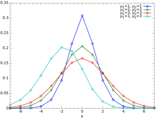
Probability mass function  Examples of the probability mass function for the Skellam distribution. The horizontal axis is the index k. (The function is only defined at integer values of k. The connecting lines do not indicate continuity.) | |||
| Parameters | |||
|---|---|---|---|
| Support | |||
| pmf | |||
| Mean | |||
| Median | N/A | ||
| Variance | |||
| Skewness | |||
| Kurtosis | |||
| MGF | |||
| CF | |||
The Skellam distribution is the discrete probability distribution of the difference of two statistically independent random variables and each Poisson-distributed with respective expected values and . It is useful in describing the statistics of the difference of two images with simple photon noise, as well as describing the point spread distribution in sports where all scored points are equal, such as baseball, hockey and soccer.
The distribution is also applicable to a special case of the difference of dependent Poisson random variables, but just the obvious case where the two variables have a common additive random contribution which is cancelled by the differencing: see Karlis & Ntzoufras (2003) for details and an application.
The probability mass function for the Skellam distribution for a difference between two independent Poisson-distributed random variables with means and is given by:
where Ik(z) is the modified Bessel function of the first kind. Since k is an integer we have that Ik(z) = I|k|(z).
Derivation
The probability mass function of a Poisson-distributed random variable with mean μ is given by
for (and zero otherwise). The Skellam probability mass function for the difference of two independent counts is the convolution of two Poisson distributions: (Skellam, 1946)
Since the Poisson distribution is zero for negative values of the count , the second sum is only taken for those terms where and . It can be shown that the above sum implies that
so that:
where I k(z) is the modified Bessel function of the first kind. The special case for is given by Irwin (1937):
Using the limiting values of the modified Bessel function for small arguments, we can recover the Poisson distribution as a special case of the Skellam distribution for .
Properties
As it is a discrete probability function, the Skellam probability mass function is normalized:
We know that the probability generating function (pgf) for a Poisson distribution is:
It follows that the pgf, , for a Skellam probability mass function will be:
Notice that the form of the probability-generating function implies that the distribution of the sums or the differences of any number of independent Skellam-distributed variables are again Skellam-distributed. It is sometimes claimed that any linear combination of two Skellam distributed variables are again Skellam-distributed, but this is clearly not true since any multiplier other than would change the support of the distribution and alter the pattern of moments in a way that no Skellam distribution can satisfy.
The moment-generating function is given by:
which yields the raw moments mk . Define:
Then the raw moments mk are
The central moments M k are
The mean, variance, skewness, and kurtosis excess are respectively:
The cumulant-generating function is given by:
which yields the cumulants:
For the special case when μ1 = μ2, an asymptotic expansion of the modified Bessel function of the first kind yields for large μ:
(Abramowitz & Stegun 1972, p. 377). Also, for this special case, when k is also large, and of order of the square root of 2μ, the distribution tends to a normal distribution:
These special results can easily be extended to the more general case of different means.
Bounds on weight above zero
If , with , then
Details can be found in Poisson distribution § Poisson races
See also
References
- Abramowitz, Milton; Stegun, Irene A., eds (June 1965). Handbook of mathematical functions with formulas, graphs, and mathematical tables (Unabridged and unaltered republ. [der Ausg.] 1964, 5. Dover printing ed.). Dover Publications. pp. 374–378. ISBN 0486612724. http://store.doverpublications.com/0486612724.html. Retrieved 27 September 2012.
- Irwin, J. O. (1937) "The frequency distribution of the difference between two independent variates following the same Poisson distribution." Journal of the Royal Statistical Society: Series A, 100 (3), 415–416. JSTOR 2980526
- Karlis, D. and Ntzoufras, I. (2003) "Analysis of sports data using bivariate Poisson models". Journal of the Royal Statistical Society, Series D, 52 (3), 381–393. doi:10.1111/1467-9884.00366
- Karlis D. and Ntzoufras I. (2006). Bayesian analysis of the differences of count data. Statistics in Medicine, 25, 1885–1905. [1]
- Skellam, J. G. (1946) "The frequency distribution of the difference between two Poisson variates belonging to different populations". Journal of the Royal Statistical Society, Series A, 109 (3), 296. JSTOR 2981372
 |
