Trace diagram

In mathematics, trace diagrams are a graphical means of performing computations in linear and multilinear algebra. They can be represented as (slightly modified) graphs in which some edges are labeled by matrices. The simplest trace diagrams represent the trace and determinant of a matrix. Several results in linear algebra, such as Cramer's Rule and the Cayley–Hamilton theorem, have simple diagrammatic proofs. They are closely related to Penrose's graphical notation.
Formal definition
Let V be a vector space of dimension n over a field F (with n≥2), and let Hom(V,V) denote the linear transformations on V. An n-trace diagram is a graph , where the sets Vi (i = 1, 2, n) are composed of vertices of degree i, together with the following additional structures:
- a ciliation at each vertex in the graph, which is an explicit ordering of the adjacent edges at that vertex;
- a labeling V2 → Hom(V,V) associating each degree-2 vertex to a linear transformation.
Note that V2 and Vn should be considered as distinct sets in the case n = 2. A framed trace diagram is a trace diagram together with a partition of the degree-1 vertices V1 into two disjoint ordered collections called the inputs and the outputs.
The "graph" underlying a trace diagram may have the following special features, which are not always included in the standard definition of a graph:
- Loops are permitted (a loop is an edge that connects a vertex to itself).
- Edges that have no vertices are permitted, and are represented by small circles.
- Multiple edges between the same two vertices are permitted.
Drawing conventions
- When trace diagrams are drawn, the ciliation on an n-vertex is commonly represented by a small mark between two of the incident edges (in the figure above, a small red dot); the specific ordering of edges follows by proceeding counter-clockwise from this mark.
- The ciliation and labeling at a degree-2 vertex are combined into a single directed node that allows one to differentiate the first edge (the incoming edge) from the second edge (the outgoing edge).
- Framed diagrams are drawn with inputs at the bottom of the diagram and outputs at the top of the diagram. In both cases, the ordering corresponds to reading from left to right.
Correspondence with multilinear functions
Every framed trace diagram corresponds to a multilinear function between tensor powers of the vector space V. The degree-1 vertices correspond to the inputs and outputs of the function, while the degree-n vertices correspond to the generalized Levi-Civita symbol (which is an anti-symmetric tensor related to the determinant). If a diagram has no output strands, its function maps tensor products to a scalar. If there are no degree-1 vertices, the diagram is said to be closed and its corresponding function may be identified with a scalar.
By definition, a trace diagram's function is computed using signed graph coloring. For each edge coloring of the graph's edges by n labels, so that no two edges adjacent to the same vertex have the same label, one assigns a weight based on the labels at the vertices and the labels adjacent to the matrix labels. These weights become the coefficients of the diagram's function.
In practice, a trace diagram's function is typically computed by decomposing the diagram into smaller pieces whose functions are known. The overall function can then be computed by re-composing the individual functions.
Examples
3-Vector diagrams
Several vector identities have easy proofs using trace diagrams. This section covers 3-trace diagrams. In the translation of diagrams to functions, it can be shown that the positions of ciliations at the degree-3 vertices has no influence on the resulting function, so they may be omitted.
It can be shown that the cross product and dot product of 3-dimensional vectors are represented by

In this picture, the inputs to the function are shown as vectors in yellow boxes at the bottom of the diagram. The cross product diagram has an output vector, represented by the free strand at the top of the diagram. The dot product diagram does not have an output vector; hence, its output is a scalar.
As a first example, consider the scalar triple product identity
To prove this diagrammatically, note that all of the following figures are different depictions of the same 3-trace diagram (as specified by the above definition):

Combining the above diagrams for the cross product and the dot product, one can read off the three leftmost diagrams as precisely the three leftmost scalar triple products in the above identity. It can also be shown that the rightmost diagram represents det[u v w]. The scalar triple product identity follows because each is a different representation of the same diagram's function.
As a second example, one can show that
(where the equality indicates that the identity holds for the underlying multilinear functions). One can show that this kind of identity does not change by "bending" the diagram or attaching more diagrams, provided the changes are consistent across all diagrams in the identity. Thus, one can bend the top of the diagram down to the bottom, and attach vectors to each of the free edges, to obtain

which reads
a well-known identity relating four 3-dimensional vectors.
Diagrams with matrices
The simplest closed diagrams with a single matrix label correspond to the coefficients of the characteristic polynomial, up to a scalar factor that depends only on the dimension of the matrix. One representation of these diagrams is shown below, where is used to indicate equality up to a scalar factor that depends only on the dimension n of the underlying vector space.
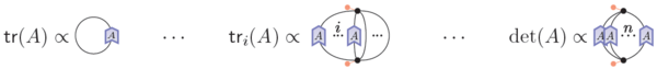 .
.

Properties
Let G be the group of n×n matrices. If a closed trace diagram is labeled by k different matrices, it may be interpreted as a function from to an algebra of multilinear functions. This function is invariant under simultaneous conjugation, that is, the function corresponding to is the same as the function corresponding to for any invertible .
Extensions and applications
Trace diagrams may be specialized for particular Lie groups by altering the definition slightly. In this context, they are sometimes called birdtracks, tensor diagrams, or Penrose graphical notation.
Trace diagrams have primarily been used by physicists as a tool for studying Lie groups. The most common applications use representation theory to construct spin networks from trace diagrams. In mathematics, they have been used to study character varieties.
See also
References
Books:
- Diagram Techniques in Group Theory, G. E. Stedman, Cambridge University Press, 1990
- Group Theory: Birdtracks, Lie's, and Exceptional Groups, Predrag Cvitanović, Princeton University Press, 2008, http://birdtracks.eu/
 |  |

