CDF-based nonparametric confidence interval
In statistics, cumulative distribution function (CDF)-based nonparametric confidence intervals are a general class of confidence intervals around statistical functionals of a distribution. To calculate these confidence intervals, all that is required is an independently and identically distributed (iid) sample from the distribution and known bounds on the support of the distribution. The latter requirement simply means that all the nonzero probability mass of the distribution must be contained in some known interval [math]\displaystyle{ [a,b] }[/math].
Intuition
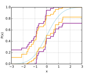
The intuition behind the CDF-based approach is that bounds on the CDF of a distribution can be translated into bounds on statistical functionals of that distribution. Given an upper and lower bound on the CDF, the approach involves finding the CDFs within the bounds that maximize and minimize the statistical functional of interest.
Properties of the bounds
Unlike approaches that make asymptotic assumptions, including bootstrap approaches and those that rely on the central limit theorem, CDF-based bounds are valid for finite sample sizes. And unlike bounds based on inequalities such as Hoeffding's and McDiarmid's inequalities, CDF-based bounds use properties of the entire sample and thus often produce significantly tighter bounds.
CDF bounds
When producing bounds on the CDF, we must differentiate between pointwise and simultaneous bands.

Pointwise band
A pointwise CDF bound is one which only guarantees their Coverage probability of [math]\displaystyle{ 1-\alpha }[/math] percent on any individual point of the empirical CDF. Because of the relaxed guarantees, these intervals can be much smaller.
One method of generating them is based on the Binomial distribution. Considering a single point of a CDF of value [math]\displaystyle{ F(x_i) }[/math], then the empirical distribution at that point will be distributed proportional to the binomial distribution with [math]\displaystyle{ p=F(x_i) }[/math] and [math]\displaystyle{ n }[/math] set equal to the number of samples in the empirical distribution. Thus, any of the methods available for generating a Binomial proportion confidence interval can be used to generate a CDF bound as well.
Simultaneous Band
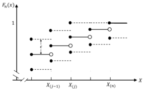
CDF-based confidence intervals require a probabilistic bound on the CDF of the distribution from which the sample were generated. A variety of methods exist for generating confidence intervals for the CDF of a distribution, [math]\displaystyle{ F }[/math], given an i.i.d. sample drawn from the distribution. These methods are all based on the empirical distribution function (empirical CDF). Given an i.i.d. sample of size n, [math]\displaystyle{ x_1,\ldots,x_n\sim F }[/math], the empirical CDF is defined to be
- [math]\displaystyle{ \hat{F}_n(t) = \frac{1}{n}\sum_{i=1}^n1\{x_i\le t\}, }[/math]
where [math]\displaystyle{ 1\{A\} }[/math] is the indicator of event A. The Dvoretzky–Kiefer–Wolfowitz inequality,[1] whose tight constant was determined by Massart,[2] places a confidence interval around the Kolmogorov–Smirnov statistic between the CDF and the empirical CDF. Given an i.i.d. sample of size n from [math]\displaystyle{ F }[/math], the bound states
- [math]\displaystyle{ P(\sup_x|F(x)-F_n(x)|\gt \varepsilon)\le2e^{-2n\varepsilon^2}. }[/math]
This can be viewed as a confidence envelope that runs parallel to, and is equally above and below, the empirical CDF.

The equally spaced confidence interval around the empirical CDF allows for different rates of violations across the support of the distribution. In particular, it is more common for a CDF to be outside of the CDF bound estimated using the Dvoretzky–Kiefer–Wolfowitz inequality near the median of the distribution than near the endpoints of the distribution. In contrast, the order statistics-based bound introduced by Learned-Miller and DeStefano[3] allows for an equal rate of violation across all of the order statistics. This in turn results in a bound that is tighter near the ends of the support of the distribution and looser in the middle of the support. Other types of bounds can be generated by varying the rate of violation for the order statistics. For example, if a tighter bound on the distribution is desired on the upper portion of the support, a higher rate of violation can be allowed at the upper portion of the support at the expense of having a lower rate of violation, and thus a looser bound, for the lower portion of the support.
A nonparametric bound on the mean
Assume without loss of generality that the support of the distribution is contained in [math]\displaystyle{ [0,1]. }[/math] Given a confidence envelope for the CDF of [math]\displaystyle{ F }[/math] it is easy to derive a corresponding confidence interval for the mean of [math]\displaystyle{ F }[/math]. It can be shown[4] that the CDF that maximizes the mean is the one that runs along the lower confidence envelope, [math]\displaystyle{ L(x) }[/math], and the CDF that minimizes the mean is the one that runs along the upper envelope, [math]\displaystyle{ U(x) }[/math]. Using the identity
- [math]\displaystyle{ E(X) = \int_0^1(1-F(x))\,dx, }[/math]
the confidence interval for the mean can be computed as
- [math]\displaystyle{ \left[\int_0^1(1-U(x))\,dx, \int_0^1(1-L(x))\,dx \right]. }[/math]
A nonparametric bound on the variance
Assume without loss of generality that the support of the distribution of interest, [math]\displaystyle{ F }[/math], is contained in [math]\displaystyle{ [0,1] }[/math]. Given a confidence envelope for [math]\displaystyle{ F }[/math], it can be shown[5] that the CDF within the envelope that minimizes the variance begins on the lower envelope, has a jump discontinuity to the upper envelope, and then continues along the upper envelope. Further, it can be shown that this variance-minimizing CDF, F', must satisfy the constraint that the jump discontinuity occurs at [math]\displaystyle{ E[F'] }[/math]. The variance maximizing CDF begins on the upper envelope, horizontally transitions to the lower envelope, then continues along the lower envelope. Explicit algorithms for calculating these variance-maximizing and minimizing CDFs are given by Romano and Wolf.[5]
Bounds on other statistical functionals
The CDF-based framework for generating confidence intervals is very general and can be applied to a variety of other statistical functionals including
- Entropy[3]
- Mutual information[6]
- Arbitrary percentiles
See also
- Bootstrapping (statistics)
- Non-parametric statistics
- Confidence interval
References
- ↑ A., Dvoretzky; Kiefer, J.; Wolfowitz, J. (1956). "Asymptotic minimax character of the sample distribution function and of the classical multinomial estimator". The Annals of Mathematical Statistics 27 (3): 642–669. doi:10.1214/aoms/1177728174.
- ↑ Massart, P. (1990). "The tight constant in the Dvoretzky–Kiefer–Wolfowitz inequality". The Annals of Probability 18 (3): 1269–1283. doi:10.1214/aop/1176990746.
- ↑ 3.0 3.1 Learned-Miller, E.; DeStefano, J. (2008). "A probabilistic upper bound on differential entropy". IEEE Transactions on Information Theory 54 (11): 5223–5230. doi:10.1109/tit.2008.929937.
- ↑ Anderson, T.W. (1969). "Confidence limits for the value of an arbitrary bounded random variable with a continuous distribution function". Bulletin of the International and Statistical Institute 43: 249–251.
- ↑ 5.0 5.1 Romano, J.P.; M., Wolf (2002). "Explicit nonparametric confidence intervals for the variance with guaranteed coverage". Communications in Statistics - Theory and Methods 31 (8): 1231–1250. doi:10.1081/sta-120006065.
- ↑ VanderKraats, N.D.; Banerjee, A. (2011). "A finite-sample, distribution-free, probabilistic lower bound on mutual information". Neural Computation 23 (7): 1862–1898. doi:10.1162/neco_a_00144. PMID 21492010.
 |

