Degree distribution
| Network science | ||||
|---|---|---|---|---|
| Network types | ||||
| Graphs | ||||
|
||||
| Models | ||||
|
||||
| ||||
In the study of graphs and networks, the degree of a node in a network is the number of connections it has to other nodes and the degree distribution is the probability distribution of these degrees over the whole network.
Definition
The degree of a node in a network (sometimes referred to incorrectly as the connectivity) is the number of connections or edges the node has to other nodes. If a network is directed, meaning that edges point in one direction from one node to another node, then nodes have two different degrees, the in-degree, which is the number of incoming edges, and the out-degree, which is the number of outgoing edges.
The degree distribution P(k) of a network is then defined to be the fraction of nodes in the network with degree k. Thus if there are n nodes in total in a network and nk of them have degree k, we have
- [math]\displaystyle{ P(k) = \frac{n_{k}}{n} }[/math].
The same information is also sometimes presented in the form of a cumulative degree distribution, the fraction of nodes with degree smaller than k, or even the complementary cumulative degree distribution, the fraction of nodes with degree greater than or equal to k (1 - C) if one considers C as the cumulative degree distribution; i.e. the complement of C.
Observed degree distributions
The degree distribution is very important in studying both real networks, such as the Internet and social networks, and theoretical networks. The simplest network model, for example, the (Erdős–Rényi model) random graph, in which each of n nodes is independently connected (or not) with probability p (or 1 − p), has a binomial distribution of degrees k:
- [math]\displaystyle{ P(k) = {n-1\choose k} p^k (1 - p)^{n-1-k}, }[/math]
(or Poisson in the limit of large n, if the average degree [math]\displaystyle{ \langle k\rangle=p(n-1) }[/math] is held fixed). Most networks in the real world, however, have degree distributions very different from this. Most are highly right-skewed, meaning that a large majority of nodes have low degree but a small number, known as "hubs", have high degree. Some networks, notably the Internet, the World Wide Web, and some social networks were argued to have degree distributions that approximately follow a power law: [math]\displaystyle{ P(k)\sim k^{-\gamma} }[/math], where γ is a constant. Such networks are called scale-free networks and have attracted particular attention for their structural and dynamical properties.[1][2][3][4] However, a survey of a wide range of real world networks suggests that scale-free networks are rare when assessed using statistically rigorous measures.[5] Some researchers have disputed these findings arguing that the definitions used in the study are inappropriately strict,[6] while others have argued that the precise functional form of the degree distribution is less important than knowing whether the degree distribution is fat-tailed or not.[7] The over-interpretation of specific forms of the degree distribution has also been criticised for failing to consider how networks may evolve over time.[8]
Excess degree distribution
Excess degree distribution is the probability distribution, for a node reached by following an edge, of the number of other edges attached to that node.[9] In other words, it is the distribution of outgoing links from a node reached by following a link.
Suppose a network has a degree distribution [math]\displaystyle{ P(k) }[/math], by selecting one node (randomly or not) and going to one of its neighbors (assuming to have one neighbor at least), then the probability of that node to have [math]\displaystyle{ k }[/math] neighbors is not given by [math]\displaystyle{ P(k) }[/math]. The reason is that, whenever some node is selected in a heterogeneous network, it is more probable to reach the hubs by following one of the existing neighbors of that node. The true probability of such nodes to have degree [math]\displaystyle{ k }[/math] is [math]\displaystyle{ q(k) }[/math] which is called the excess degree of that node. In the configuration model, which correlations between the nodes have been ignored and every node is assumed to be connected to any other nodes in the network with the same probability, the excess degree distribution can be found as:[9]
[math]\displaystyle{ q(k) = \frac{k+1}{\langle k \rangle}P(k+1), }[/math]
where [math]\displaystyle{ {\langle k \rangle} }[/math] is the mean-degree (average degree) of the model. It follows to that fact that the average degree of the neighbor of any node is greater than the average degree of that node. In social networks, it mean that your friends, on average, have more friends than you. This is famous as the friendship paradox. It can be shown that a network can have a giant component, if its average excess degree is larger than one:
[math]\displaystyle{ \sum_k kq(k) \gt 1 \Rightarrow {\langle k^2 \rangle}/{\langle k \rangle} - 1 \gt 1 \Rightarrow {\langle k^2 \rangle}-2{\langle k \rangle}\gt 0 }[/math]
Bear in mind that the last two equations are just for the configuration model and to derive the excess degree distribution of a real-word network, we should also add degree correlations into account.[9]
Generating functions method
Generating functions can be used to calculate different properties of random networks. Given the degree distribution and the excess degree distribution of some network, [math]\displaystyle{ P(k) }[/math] and [math]\displaystyle{ q(k) }[/math] respectively, it is possible to write two power series in the following forms:
[math]\displaystyle{ G_0(x) = \textstyle \sum_{k} \displaystyle P(k)x^k }[/math] and [math]\displaystyle{ G_1(x) = \textstyle \sum_{k} \displaystyle q(k)x^k = \textstyle \sum_{k} \displaystyle \frac{k}{\langle k \rangle}P(k)x^{k-1} }[/math]
[math]\displaystyle{ G_1(x) }[/math] can also be obtained from derivatives of [math]\displaystyle{ G_0(x) }[/math]:
[math]\displaystyle{ G_1(x) = \frac{G'_0(x)}{G'_0(1)} }[/math]
If we know the generating function for a probability distribution [math]\displaystyle{ P(k) }[/math] then we can recover the values of [math]\displaystyle{ P(k) }[/math] by differentiating:
[math]\displaystyle{ P(k) = \frac{1}{k!} {\operatorname{d}^k\!G\over\operatorname{d}\!x^k}\biggl \vert _{x=0} }[/math]
Some properties, e.g. the moments, can be easily calculated from [math]\displaystyle{ G_0(x) }[/math] and its derivatives:
- [math]\displaystyle{ {\langle k \rangle} = G'_0(1) }[/math]
- [math]\displaystyle{ {\langle k^2 \rangle} = G''_0(1) + G'_0(1) }[/math]
And in general:[9]
- [math]\displaystyle{ {\langle k^m \rangle} = \Biggl[{\bigg(\operatorname{x}{\operatorname{d}\!\over\operatorname{dx}\!}\biggl)^m}G_0(x)\Biggl]_{x=1} }[/math]
For Poisson-distributed random networks, such as the ER graph, [math]\displaystyle{ G_1(x) = G_0(x) }[/math], that is the reason why the theory of random networks of this type is especially simple. The probability distributions for the 1st and 2nd-nearest neighbors are generated by the functions [math]\displaystyle{ G_0(x) }[/math] and [math]\displaystyle{ G_0(G_1(x)) }[/math]. By extension, the distribution of [math]\displaystyle{ m }[/math]-th neighbors is generated by:
[math]\displaystyle{ G_0\bigl(G_1(...G_1(x)...)\bigr) }[/math], with [math]\displaystyle{ m-1 }[/math] iterations of the function [math]\displaystyle{ G_1 }[/math] acting on itself.[10]
The average number of 1st neighbors, [math]\displaystyle{ c_1 }[/math], is [math]\displaystyle{ {\langle k \rangle} = {dG_0(x)\over dx}|_{x=1} }[/math] and the average number of 2nd neighbors is: [math]\displaystyle{ c_2 = \biggl[ {d\over dx}G_0\big(G_1(x)\big)\biggl]_{x=1} = G_1'(1)G'_0\big(G_1(1)\big) = G_1'(1)G'_0(1) = G''_0(1) }[/math]
Degree distribution for directed networks
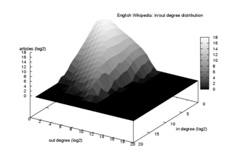
In a directed network, each node has some in-degree [math]\displaystyle{ k_{ in} }[/math] and some out-degree [math]\displaystyle{ k_{out} }[/math] which are the number of links which have run into and out of that node respectfully. If [math]\displaystyle{ P(k_{in}, k_{out}) }[/math] is the probability that a randomly chosen node has in-degree [math]\displaystyle{ k_{ in} }[/math] and out-degree [math]\displaystyle{ k_{out} }[/math] then the generating function assigned to this joint probability distribution can be written with two valuables [math]\displaystyle{ x }[/math] and [math]\displaystyle{ y }[/math] as:
[math]\displaystyle{ \mathcal{G}(x,y) = \sum_{k_{in},k_{out}} \displaystyle P({k_{in},k_{out}})x^{k_{in}}y^{k_{out}} . }[/math]
Since every link in a directed network must leave some node and enter another, the net average number of links entering a node is zero. Therefore,
[math]\displaystyle{ \langle{k_{in}-k_{out}}\rangle =\sum_{k_{in},k_{out}} \displaystyle (k_{in}-k_{out})P({k_{in},k_{out}}) = 0 }[/math],
which implies that, the generation function must satisfy:
[math]\displaystyle{ {\partial \mathcal{G}\over\partial x}\vert _{x,y=1} = {\partial \mathcal{G}\over\partial y}\vert _{x,y=1} = c, }[/math]
where [math]\displaystyle{ c }[/math] is the mean degree (both in and out) of the nodes in the network; [math]\displaystyle{ \langle{k_{in}}\rangle = \langle{k_{out}}\rangle = c. }[/math]
Using the function [math]\displaystyle{ \mathcal{G}(x,y) }[/math], we can again find the generation function for the in/out-degree distribution and in/out-excess degree distribution, as before. [math]\displaystyle{ G^{in}_0(x) }[/math] can be defined as generating functions for the number of arriving links at a randomly chosen node, and [math]\displaystyle{ G^{in}_1(x) }[/math]can be defined as the number of arriving links at a node reached by following a randomly chosen link. We can also define generating functions [math]\displaystyle{ G^{out}_0(y) }[/math] and [math]\displaystyle{ G^{out}_1(y) }[/math] for the number leaving such a node:[10]
- [math]\displaystyle{ G^{in}_0(x) = \mathcal{G}(x,1) }[/math]
- [math]\displaystyle{ G^{in}_1(x) = \frac{1}{c} {\partial \mathcal{G}\over\partial x}\vert _{y=1} }[/math]
- [math]\displaystyle{ G^{out}_0(y) = \mathcal{G}(1,y) }[/math]
- [math]\displaystyle{ G^{out}_1(y) = \frac{1}{c} {\partial \mathcal{G}\over\partial y}\vert _{x=1} }[/math]
Here, the average number of 1st neighbors, [math]\displaystyle{ c }[/math], or as previously introduced as [math]\displaystyle{ c_1 }[/math], is [math]\displaystyle{ {\partial \mathcal{G}\over\partial x}\biggl \vert _{x,y=1} = {\partial \mathcal{G}\over\partial y}\biggl \vert _{x,y=1} }[/math] and the average number of 2nd neighbors reachable from a randomly chosen node is given by: [math]\displaystyle{ c_2 = G_1'(1)G'_0(1) ={\partial^2 \mathcal{G}\over\partial x\partial y}\biggl \vert _{x,y=1} }[/math]. These are also the numbers of 1st and 2nd neighbors from which a random node can be reached, since these equations are manifestly symmetric in [math]\displaystyle{ x }[/math] and [math]\displaystyle{ y }[/math].[10]
Degree distribution for signed networks
In a signed network, each node has a positive-degree [math]\displaystyle{ k_{ +} }[/math] and a negative degree [math]\displaystyle{ k_{-} }[/math] which are the positive number of links and negative number of links connected to that node respectfully. So [math]\displaystyle{ P(k_{+}) }[/math] and [math]\displaystyle{ P(k_{-}) }[/math] denote negative degree distribution and positive degree distribution of the signed network.[11][12]
See also
References
- ↑ Barabási, Albert-László; Albert, Réka (1999-10-15). "Emergence of Scaling in Random Networks". Science 286 (5439): 509–512. doi:10.1126/science.286.5439.509. ISSN 0036-8075. PMID 10521342. Bibcode: 1999Sci...286..509B.
- ↑ Albert, Réka; Barabási, Albert-László (2000-12-11). "Topology of Evolving Networks: Local Events and Universality". Physical Review Letters 85 (24): 5234–5237. doi:10.1103/physrevlett.85.5234. ISSN 0031-9007. PMID 11102229. Bibcode: 2000PhRvL..85.5234A. https://repository.library.northeastern.edu/files/neu:331099/fulltext.pdf. Retrieved 2019-09-25.
- ↑ Dorogovtsev, S. N.; Mendes, J. F. F.; Samukhin, A. N. (2001-05-21). "Size-dependent degree distribution of a scale-free growing network". Physical Review E 63 (6): 062101. doi:10.1103/physreve.63.062101. ISSN 1063-651X. PMID 11415146. Bibcode: 2001PhRvE..63f2101D.
- ↑ Pachon, Angelica; Sacerdote, Laura; Yang, Shuyi (2018). "Scale-free behavior of networks with the copresence of preferential and uniform attachment rules". Physica D: Nonlinear Phenomena 371: 1–12. doi:10.1016/j.physd.2018.01.005. Bibcode: 2018PhyD..371....1P.
- ↑ Broido, Anna D.; Clauset, Aaron (2019-03-04). "Scale-free networks are rare" (in en). Nature Communications 10 (1): 1017. doi:10.1038/s41467-019-08746-5. ISSN 2041-1723. PMID 30833554.
- ↑ Voitalov, Ivan; van der Hoorn, Pim; van der Hofstad, Remco; Krioukov, Dmitri (18 October 2019). "Scale-free networks well done". Physical Review Research 1 (3): 033034. doi:10.1103/PhysRevResearch.1.033034.
- ↑ Holme, Petter (2019-03-04). "Rare and everywhere: Perspectives on scale-free networks" (in en). Nature Communications 10 (1): 1016. doi:10.1038/s41467-019-09038-8. ISSN 2041-1723. PMID 30833568. Bibcode: 2019NatCo..10.1016H.
- ↑ Falkenberg, Max; Lee, Jong-Hyeok; Amano, Shun-ichi; Ogawa, Ken-ichiro; Yano, Kazuo; Miyake, Yoshihiro; Evans, Tim S.; Christensen, Kim (18 June 2020). "Identifying time dependence in network growth". Physical Review Research 2 (2): 023352. doi:10.1103/PhysRevResearch.2.023352.
- ↑ 9.0 9.1 9.2 9.3 Newman, Mark (2018-10-18) (in en). Networks. 1. Oxford University Press. doi:10.1093/oso/9780198805090.001.0001. ISBN 978-0-19-880509-0. http://www.oxfordscholarship.com/view/10.1093/oso/9780198805090.001.0001/oso-9780198805090. Retrieved 2020-04-19.
- ↑ 10.0 10.1 10.2 Newman, M. E. J.; Strogatz, S. H.; Watts, D. J. (2001-07-24). "Random graphs with arbitrary degree distributions and their applications" (in en). Physical Review E 64 (2): 026118. doi:10.1103/PhysRevE.64.026118. ISSN 1063-651X. PMID 11497662.
- ↑ "Topological impact of negative links on the stability of resting-state brain network". Scientific Reports 11 (1): 2176. January 2021. doi:10.1038/s41598-021-81767-7. PMID 33500525.
- ↑ "Degree correlations in signed social networks". Physica A: Statistical Mechanics and Its Applications 422: 25–39. 2015. doi:10.1016/j.physa.2014.11.062. https://www.sciencedirect.com/science/article/abs/pii/S0378437114010334. Retrieved 2021-02-10.
- Albert, R.; Barabasi, A.-L. (2002). "Statistical mechanics of complex networks". Reviews of Modern Physics 74 (1): 47–97. doi:10.1103/RevModPhys.74.47. Bibcode: 2002RvMP...74...47A.
- Dorogovtsev, S.; Mendes, J. F. F. (2002). "Evolution of networks". Advances in Physics 51 (4): 1079–1187. doi:10.1080/00018730110112519. Bibcode: 2002AdPhy..51.1079D.
- Newman, M. E. J. (2003). "The structure and function of complex networks". SIAM Review 45 (2): 167–256. doi:10.1137/S003614450342480. Bibcode: 2003SIAMR..45..167N.
 |


