Hotelling's T-squared distribution
|
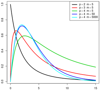
Probability density function  | |||
|
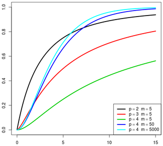
Cumulative distribution function  | |||
| Parameters |
p - dimension of the random variables m - related to the sample size | ||
|---|---|---|---|
| Support |
[math]\displaystyle{ x \in (0, +\infty)\; }[/math] if [math]\displaystyle{ p = 1 }[/math] [math]\displaystyle{ x \in [0, +\infty)\; }[/math] otherwise. | ||
In statistics, particularly in hypothesis testing, the Hotelling's T-squared distribution (T2), proposed by Harold Hotelling,[1] is a multivariate probability distribution that is tightly related to the F-distribution and is most notable for arising as the distribution of a set of sample statistics that are natural generalizations of the statistics underlying the Student's t-distribution. The Hotelling's t-squared statistic (t2) is a generalization of Student's t-statistic that is used in multivariate hypothesis testing.[2]
Motivation
The distribution arises in multivariate statistics in undertaking tests of the differences between the (multivariate) means of different populations, where tests for univariate problems would make use of a t-test. The distribution is named for Harold Hotelling, who developed it as a generalization of Student's t-distribution.[1]
Definition
If the vector [math]\displaystyle{ d }[/math] is Gaussian multivariate-distributed with zero mean and unit covariance matrix [math]\displaystyle{ N(\mathbf{0}_{p}, \mathbf{I}_{p, p}) }[/math] and [math]\displaystyle{ M }[/math] is a [math]\displaystyle{ p \times p }[/math] matrix with unit scale matrix and m degrees of freedom with a Wishart distribution [math]\displaystyle{ W(\mathbf{I}_{p, p}, m) }[/math], then the quadratic form [math]\displaystyle{ X }[/math] has a Hotelling distribution (with parameters [math]\displaystyle{ p }[/math] and [math]\displaystyle{ m }[/math]):[3]
- [math]\displaystyle{ X = m d^T M^{-1} d \sim T^2(p, m). }[/math]
Furthermore, if a random variable X has Hotelling's T-squared distribution, [math]\displaystyle{ X \sim T^2_{p,m} }[/math], then:[1]
- [math]\displaystyle{ \frac{m-p+1}{pm} X\sim F_{p,m-p+1} }[/math]
where [math]\displaystyle{ F_{p,m-p+1} }[/math] is the F-distribution with parameters p and m−p+1.
Hotelling t-squared statistic
Let [math]\displaystyle{ \hat{\mathbf \Sigma} }[/math] be the sample covariance:
- [math]\displaystyle{ \hat{\mathbf \Sigma} = \frac 1 {n-1} \sum_{i=1}^n (\mathbf{x}_i -\overline{\mathbf{x}}) (\mathbf{x}_i-\overline{\mathbf{x}})' }[/math]
where we denote transpose by an apostrophe. It can be shown that [math]\displaystyle{ \hat{\mathbf \Sigma} }[/math] is a positive (semi) definite matrix and [math]\displaystyle{ (n-1)\hat{\mathbf \Sigma} }[/math] follows a p-variate Wishart distribution with n−1 degrees of freedom.[4] The sample covariance matrix of the mean reads [math]\displaystyle{ \hat{\mathbf \Sigma}_\overline{\mathbf x}=\hat{\mathbf \Sigma}/n }[/math].
The Hotelling's t-squared statistic is then defined as:[5]
- [math]\displaystyle{ t^2=(\overline{\mathbf x}-\boldsymbol{\mu})'\hat{\mathbf \Sigma}_\overline{\mathbf x}^{-1} (\overline{\mathbf x}-\boldsymbol{\mathbf\mu}), }[/math]
which is proportional to the distance between the sample mean and [math]\displaystyle{ \boldsymbol{\mu} }[/math]. Because of this, one should expect the statistic to assume low values if [math]\displaystyle{ \overline{\mathbf x} \approx \boldsymbol{\mu} }[/math], and high values if they are different.
From the distribution,
- [math]\displaystyle{ t^2 \sim T^2_{p,n-1}=\frac{p(n-1)}{n-p} F_{p,n-p} , }[/math]
where [math]\displaystyle{ F_{p,n-p} }[/math] is the F-distribution with parameters p and n − p.
In order to calculate a p-value (unrelated to p variable here), note that the distribution of [math]\displaystyle{ t^2 }[/math] equivalently implies that
- [math]\displaystyle{ \frac{n-p} {p(n-1)} t^2 \sim F_{p,n-p} . }[/math]
Then, use the quantity on the left hand side to evaluate the p-value corresponding to the sample, which comes from the F-distribution. A confidence region may also be determined using similar logic.
Motivation
Let [math]\displaystyle{ \mathcal{N}_p(\boldsymbol{\mu},{\mathbf \Sigma}) }[/math] denote a p-variate normal distribution with location [math]\displaystyle{ \boldsymbol{\mu} }[/math] and known covariance [math]\displaystyle{ {\mathbf \Sigma} }[/math]. Let
- [math]\displaystyle{ {\mathbf x}_1,\dots,{\mathbf x}_n\sim \mathcal{N}_p(\boldsymbol{\mu},{\mathbf \Sigma}) }[/math]
be n independent identically distributed (iid) random variables, which may be represented as [math]\displaystyle{ p\times1 }[/math] column vectors of real numbers. Define
- [math]\displaystyle{ \overline{\mathbf x}=\frac{\mathbf{x}_1+\cdots+\mathbf{x}_n}{n} }[/math]
to be the sample mean with covariance [math]\displaystyle{ {\mathbf \Sigma}_\overline{\mathbf x}={\mathbf \Sigma}/ n }[/math]. It can be shown that
- [math]\displaystyle{ (\overline{\mathbf x}-\boldsymbol{\mu})'{\mathbf \Sigma}_\overline{\mathbf x}^{-1}(\overline{\mathbf x}-\boldsymbol{\mathbf\mu})\sim\chi^2_p , }[/math]
where [math]\displaystyle{ \chi^2_p }[/math] is the chi-squared distribution with p degrees of freedom.[6]
Proof
|
|---|
|
Proof To show this use the fact that [math]\displaystyle{ \overline{\mathbf x}\sim \mathcal{N}_p(\boldsymbol{\mu},{\mathbf \Sigma}/n) }[/math] and derive the characteristic function of the random variable [math]\displaystyle{ \mathbf y = (\bar{\mathbf x}-\boldsymbol{\mu})'{\mathbf \Sigma}_\bar{\mathbf x}^{-1}(\bar{\mathbf x}-\boldsymbol{\mathbf\mu}) = (\bar{\mathbf x}-\boldsymbol{\mu})'({\mathbf \Sigma} / n)^{-1}(\bar{\mathbf x}-\boldsymbol{\mathbf\mu}) }[/math]. As usual, let [math]\displaystyle{ | \cdot | }[/math] denote the determinant of the argument, as in [math]\displaystyle{ | \boldsymbol\Sigma | }[/math]. By definition of characteristic function, we have:[7]
There are two exponentials inside the integral, so by multiplying the exponentials we add the exponents together, obtaining:
Now take the term [math]\displaystyle{ |\boldsymbol\Sigma/n|^{-1/2} }[/math] off the integral, and multiply everything by an identity [math]\displaystyle{ I = |(\boldsymbol\Sigma^{-1}-2 i \theta \boldsymbol\Sigma^{-1})^{-1} / n|^{1/2} \;\cdot\; |(\boldsymbol\Sigma^{-1}-2 i \theta \boldsymbol\Sigma^{-1})^{-1} / n|^{-1/2} }[/math], bringing one of them inside the integral:
But the term inside the integral is precisely the probability density function of a multivariate normal distribution with covariance matrix [math]\displaystyle{ (\boldsymbol\Sigma^{-1}-2 i \theta \boldsymbol\Sigma^{-1})^{-1} / n = \left[ n (\boldsymbol\Sigma^{-1}-2 i \theta \boldsymbol\Sigma^{-1}) \right]^{-1} }[/math] and mean [math]\displaystyle{ \mu }[/math], so when integrating over all [math]\displaystyle{ x_1, \dots, x_p }[/math], it must yield [math]\displaystyle{ 1 }[/math] per the probability axioms.[clarification needed] We thus end up with:
where [math]\displaystyle{ I_p }[/math] is an identity matrix of dimension [math]\displaystyle{ p }[/math]. Finally, calculating the determinant, we obtain:
which is the characteristic function for a chi-square distribution with [math]\displaystyle{ p }[/math] degrees of freedom. [math]\displaystyle{ \;\;\;\blacksquare }[/math] |
Two-sample statistic
If [math]\displaystyle{ {\mathbf x}_1,\dots,{\mathbf x}_{n_x}\sim N_p(\boldsymbol{\mu},{\mathbf \Sigma}) }[/math] and [math]\displaystyle{ {\mathbf y}_1,\dots,{\mathbf y}_{n_y}\sim N_p(\boldsymbol{\mu},{\mathbf \Sigma}) }[/math], with the samples independently drawn from two independent multivariate normal distributions with the same mean and covariance, and we define
- [math]\displaystyle{ \overline{\mathbf x}=\frac{1}{n_x}\sum_{i=1}^{n_x} \mathbf{x}_i \qquad \overline{\mathbf y}=\frac{1}{n_y}\sum_{i=1}^{n_y} \mathbf{y}_i }[/math]
as the sample means, and
- [math]\displaystyle{ \hat{\mathbf \Sigma}_{\mathbf x}=\frac{1}{n_x-1}\sum_{i=1}^{n_{x}} (\mathbf{x}_i-\overline{\mathbf x})(\mathbf{x}_i-\overline{\mathbf x})' }[/math]
- [math]\displaystyle{ \hat{\mathbf \Sigma}_{\mathbf y}=\frac{1}{n_y-1}\sum_{i=1}^{n_{y}} (\mathbf{y}_i-\overline{\mathbf y})(\mathbf{y}_i-\overline{\mathbf y})' }[/math]
as the respective sample covariance matrices. Then
- [math]\displaystyle{ \hat{\mathbf \Sigma}= \frac{(n_x - 1) \hat{\mathbf \Sigma}_{\mathbf x} + (n_y - 1) \hat{\mathbf \Sigma}_{\mathbf y}}{n_x+n_y-2} }[/math]
is the unbiased pooled covariance matrix estimate (an extension of pooled variance).
Finally, the Hotelling's two-sample t-squared statistic is
- [math]\displaystyle{ t^2 = \frac{n_x n_y}{n_x+n_y}(\overline{\mathbf x}-\overline{\mathbf y})'\hat{\mathbf \Sigma}^{-1}(\overline{\mathbf x}-\overline{\mathbf y}) \sim T^2(p, n_x+n_y-2) }[/math]
Related concepts
It can be related to the F-distribution by[4]
- [math]\displaystyle{ \frac{n_x+n_y-p-1}{(n_x+n_y-2)p}t^2 \sim F(p,n_x+n_y-1-p). }[/math]
The non-null distribution of this statistic is the noncentral F-distribution (the ratio of a non-central Chi-squared random variable and an independent central Chi-squared random variable)
- [math]\displaystyle{ \frac{n_x+n_y-p-1}{(n_x+n_y-2)p}t^2 \sim F(p,n_x+n_y-1-p;\delta), }[/math]
with
- [math]\displaystyle{ \delta = \frac{n_x n_y}{n_x+n_y}\boldsymbol{d}'\mathbf{\Sigma}^{-1}\boldsymbol{d}, }[/math]
where [math]\displaystyle{ \boldsymbol{d}=\mathbf{\overline{x} - \overline{y}} }[/math] is the difference vector between the population means.
In the two-variable case, the formula simplifies nicely allowing appreciation of how the correlation, [math]\displaystyle{ \rho }[/math], between the variables affects [math]\displaystyle{ t^2 }[/math]. If we define
- [math]\displaystyle{ d_{1} = \overline{x}_{1}-\overline{y}_{1}, \qquad d_{2} = \overline{x}_{2}-\overline{y}_{2} }[/math]
and
- [math]\displaystyle{ s_1 = \sqrt{\Sigma_{11}} \qquad s_2 = \sqrt{\Sigma_{22}} \qquad \rho = \Sigma_{12}/(s_1 s_2) = \Sigma_{21}/(s_1 s_2) }[/math]
then
- [math]\displaystyle{ t^2 = \frac{n_x n_y}{(n_x+n_y)(1-r^2)} \left [ \left ( \frac{d_1}{s_1} \right )^2+\left ( \frac{d_2}{s_2} \right )^2-2\rho \left ( \frac{d_1}{s_1} \right )\left ( \frac{d_2}{s_2} \right ) \right ] }[/math]
Thus, if the differences in the two rows of the vector [math]\displaystyle{ \mathbf d = \overline{\mathbf x}-\overline{\mathbf y} }[/math] are of the same sign, in general, [math]\displaystyle{ t^2 }[/math] becomes smaller as [math]\displaystyle{ \rho }[/math] becomes more positive. If the differences are of opposite sign [math]\displaystyle{ t^2 }[/math] becomes larger as [math]\displaystyle{ \rho }[/math] becomes more positive.
A univariate special case can be found in Welch's t-test.
More robust and powerful tests than Hotelling's two-sample test have been proposed in the literature, see for example the interpoint distance based tests which can be applied also when the number of variables is comparable with, or even larger than, the number of subjects.[8][9]
See also
- Student's t-test in univariate statistics
- Student's t-distribution in univariate probability theory
- Multivariate Student distribution
- F-distribution (commonly tabulated or available in software libraries, and hence used for testing the T-squared statistic using the relationship given above)
- Wilks's lambda distribution (in multivariate statistics, Wilks's Λ is to Hotelling's T2 as Snedecor's F is to Student's t in univariate statistics)
References
- ↑ 1.0 1.1 1.2 "The generalization of Student's ratio". Annals of Mathematical Statistics 2 (3): 360–378. 1931. doi:10.1214/aoms/1177732979.
- ↑ Johnson, R.A.; Wichern, D.W. (2002). Applied multivariate statistical analysis. 5. Prentice hall.
- ↑ Eric W. Weisstein, MathWorld
- ↑ 4.0 4.1 Mardia, K. V.; Kent, J. T.; Bibby, J. M. (1979). Multivariate Analysis. Academic Press. ISBN 978-0-12-471250-8.
- ↑ "6.5.4.3. Hotelling's T squared". http://www.itl.nist.gov/div898/handbook/pmc/section5/pmc543.htm.
- ↑ End of chapter 4.2 of Johnson, R.A. & Wichern, D.W. (2002)
- ↑ Billingsley, P. (1995). "26. Characteristic Functions". Probability and measure (3rd ed.). Wiley. ISBN 978-0-471-00710-4.
- ↑ Marozzi, M. (2016). "Multivariate tests based on interpoint distances with application to magnetic resonance imaging". Statistical Methods in Medical Research 25 (6): 2593–2610. doi:10.1177/0962280214529104. PMID 24740998.
- ↑ Marozzi, M. (2015). "Multivariate multidistance tests for high-dimensional low sample size case-control studies". Statistics in Medicine 34 (9): 1511–1526. doi:10.1002/sim.6418. PMID 25630579.
External links
- Hazewinkel, Michiel, ed. (2001), "Hotelling T2-distribution", Encyclopedia of Mathematics, Springer Science+Business Media B.V. / Kluwer Academic Publishers, ISBN 978-1-55608-010-4, https://www.encyclopediaofmath.org/index.php?title=H/h048070
 |

