Software:COHERENS
| Developer(s) | Royal Belgian Institute of Natural Sciences, led by Patrick Luyten |
|---|---|
| Stable release | 2.11
/ July 17, 2017 |
| Written in | Fortran 90 |
| Operating system | Linux |
| Type | Computer simulation |
| License | European Union Public Licence |
| Website | odnature |
COHERENS is an open-source hydrodynamic computer model for shallow waters[1]. It was developed in the 1990s by the Royal Belgian Institute of Natural Sciences (RBINS). The name COHERENS is an acronym of COupled Hydrodynamical Ecological model for REgioNal Shelf seas. COHERENS can be used in 1D, 2D or 3D mode and can model both salt waters such as coastal and shelf seas and freshwater basins such as lakes. Applications of the model include obtaining a better understanding of shallow water systems [2] and managing pollution[3][4].
History
The initial version of the model (COHERENS V1) has been developed since 1990 and was first released as an open-source code in April 2000[1][5]. The project was funded by the European Union and the group of developers consisted of scientists from multiple countries and institutes in the EU and the Operational Directorate Natural Environment (OD Nature), which at that time was called the Management Unit of the North Sea Mathematical Models (MUMM)) and is a department of the RBINS. This first version of COHERENS was written in Fortran 77 and had four major modules[1]: A physical part for solving advection and diffusion, a microbiological module for dealing with the dynamics of microplankton, detritus, dissolved inorganic nitrogen and oxygen, a sediment module for modelling deposition and resuspension of particles, and a module for Eulerian and Lagrangian transport that could model the distribution of a pollutant.
Work on a new version, COHERENS V2.0, started in 2003 and was finished in 2009. This development was part of the EU Fifth and Sixth Framework Programmes. This second version only contains a physical component, but has several new and improved implementations, such as additional types of open boundary conditions, turbulence schemes, and more flexible model grids. Furthermore, it was re-written in Fortran 90.
From 2008 to 2015 the second version of the model was further developed on commission of the Maritime Access division Department of Mobility and Public Works of the Flemish Government. The developments were part of a project with the goal of expanding the numerical modelling tools for the North Sea harbors[6]. Several parties were involved: IMDC, Antea Group, Gent University, and Leuven University. The main additions and adaptations include the introduction of modules for sediment transport and morphology, dredging operations, and structures for engineering applications. Furthermore, a Central Input File (CIF) was added to make the code more accessible to users who are not familiar with the Fortran 90 programming language.
There are now more than 2100 registered users in 109 different countries. The countries with most users are China and Iran.
Access
The model’s source code is public domain under the European Union Public Licence (EUPL)[7]. It is therefore free to use and to modify. After registration on the website, COHERENS will be available to download. There is a comprehensive manual available that starts with an introduction to Linux and helps with installing and compiling COHERENS. There are also several test cases available[8].
Framework and user options
COHERENS has a variety of different options. The default settings allow the user to run the model without detailed knowledge of the scientific basis[1]. Furthermore, there are “switches” that can be used to select the desired options. An alternative to changing the model code to setup the model is using the Central Input File (CIF). This file can be edited in a text editor and makes knowledge of the Fortran 90 programming language unnecessary. For users with more programming experience, the modularity of the program allows users to replace modules without affecting the core of the program.
Model grid
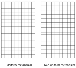
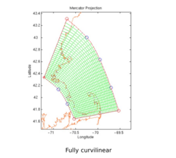
The full model is 3D, but it can be set up in a depth-averaged mode to make it 2D, and in a water column mode which is 1D[9]. For the horizontal there is the choice between a uniform rectangular, a non-uniform rectangular or a curvilinear grid.
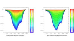
For the vertical, the model uses the sigma coordinate system. There are three options: uniform, non-uniform vertically and non-uniform in both vertical and horizontal directions (s-coordinates).
The discretization of the model equations is done on an Arakawa C-grid, with the choice of either a Cartesian or a spherical coordinate system. Cartesian coordinates allow for an easier setup in the horizontal grid if the size of the area under consideration is limited such that the Earth’s curvature is negligible, and the Coriolis frequency can be assumed to be constant in space.
Physics
In 3D mode the equations that make up the physical backbone of the model are the continuity equation, the momentum equations, and equation of state that describe the potential temperature and the salinity[9]. In the default of the program the equations are simplified with the following approximations[6]:
- The Boussinesq approximation
- The hydrostatic approximation.
- The traditional approximation; the horizontal component of the Earth’s rotation vector is zero. This approximation is invalid for non-hydrostatic water masses or for low latitudes[9].
Horizontal diffusion is implemented using constant diffusion coefficients or the Smagorinsky (1963) parameterizations[10]. For vertical diffusion there is a variety of turbulence schemes available, where the use of RANS equations is the most complex option.
The default of the model is to exclude density effects (barotropic mode), but there are also different options to run the model in baroclinic mode[9]. The density effects on the momentum and turbulence equations are then included in the equation of state, where different options can be chosen: a linear equation of state or a non-linear equation of state with a zero or a non-zero pressure.
In 2D mode it is assumed that there is no dependence on depth, and all 3D currents and scalar quantities are depth-averaged. The 3D continuity and momentum equations are supplemented by additional 2D equations for the depth integrated current and the surface elevation[9].
In 1D mode the vertical is the only axis, and the horizontal grid is reduced to a singular point. Simplifications include that advective and horizontal diffusion terms are set to zero, the horizontal pressure gradient is neglected except for the barotropic surface slope term, and the continuity equation is not solved[9].
Other features
- Hydraulic structures
- Drying and wetting to simulate for example inundation of land.
- Dredging and relocation
- Morphology of the sediment beds
- Sediment transport
- Absorption of solar radiation
- Tidal forcing
Boundary conditions
At the surface and at the bottom Neumann boundary conditions or Dirichlet boundary conditions are applied[9]. For the surface drag and exchange coefficients there are several options, ranging in complexity from a constant value to depending on the wind speed, the air-sea temperature difference, and the relative humidity. For the currents at the bottom there are different stress conditions to choose from. Lateral boundary conditions can be open.
Parallel processing
To speed up the computations and distribute internal memory over different processes, the Message Passing Interface (MPI) communication library can be used.
Output
The model can give three types of output, for user specified variables: Time series, time averaged output, and harmonic output[11]. Harmonic analysis needs to be enabled and the output can consist of residuals, amplitudes, phases, and elliptic parameters. Apart from the output itself, the output files contain the coordinates of the output grid and metadata such as the setup parameters. Output files are in ASCII or netCDF format.
See also
- General circulation model
- Ocean general circulation model
- List of ocean circulation models
- Climate model
- Oceanography
- Physical oceanography
References
- ↑ 1.0 1.1 1.2 1.3 Luyten, Patrick. "COHERENS Manual Chapter 1 General Overview". OD Nature. https://odnature.naturalsciences.be/downloads/coherens/documentation/chapter1.pdf.
- ↑ Mehrfar, Hesameddin; Azad, Masoud Torabi; Lari, Kamran; Bidokhti, Abbasali Aliakbari (1 January 2020). "Seasonal Variations of the Coastal Currents and Eddies in the Persian Gulf: A Numerical Case Study". Marine Technology Society Journal 54 (1): 44–52.
- ↑ Hassanzadeh, Smaeyl; Hajrasouliha, Omid; Latifi, Ali Rezaei (28 July 2016). "The Role of Wind in Modeling of Oil Pollution Transport and Diffusion in the Persian Gulf" (in en). Environmental Modeling & Assessment 21 (6): 721–730. doi:10.1007/s10666-016-9526-2. ISSN 1420-2026.
- ↑ Mestres, M.; Sierra, J.P.; Pascual, A.; Mösso, C.; Río, J. González del; Rodilla, M. (2009). "Bacterial pollution in Cullera Bay (Spanish Mediterranean coast)". Journal of Coastal Research: 861–865. ISSN 0749-0208. https://www.jstor.org/stable/25737701.
- ↑ Luyten, Patrick. "COHERENS - A Coupled Hydrodynamical Ecological Model for Regional and Shelf Seas: User Documentation. Version 2.1.2.". RBINS-MUMM Report, Royal Belgian Institute of Natural Sciences. https://www.scribd.com/document/403861084/CoherensBook-pdf.
- ↑ 6.0 6.1 THV IMDC-Soresma (9 August 2012). Task order 4: Design of the implicit scheme in COHERENS (Report). Antwerp, Belgium: Afdeling Maritime Toegang. https://www.scribd.com/document/323030643/257356.
- ↑ "About COHERENS, Licence". OD Nature. http://odnature.naturalsciences.be/coherens/about#licence.
- ↑ "Test cases". OD Nature. http://odnature.naturalsciences.be/coherens/test-cases.
- ↑ 9.0 9.1 9.2 9.3 9.4 9.5 9.6 Luyten, Patrick. "COHERENS Manual Chapter 4 Physical Model". OD Nature. https://odnature.naturalsciences.be/downloads/coherens/documentation/chapter4.pdf.
- ↑ Smagorinsky, J. (1963). "General circulation experiments with the primitive equations - I. The basic experiment". Monthly Weather Review 91 (3): 99-164. doi:10.1175/1520-0493(1963)091<0099:GCEWTP>2.3.CO;2.
- ↑ Luyten, Patrick. "COHERENS Manual Chapter 9 Model Input and Output". OD Nature. https://odnature.naturalsciences.be/downloads/coherens/documentation/chapter9.pdf.
External links


