Parameterization in a weather or climate model in the context of numerical weather prediction is a method of replacing processes that are too small-scale or complex to be physically represented in the model by a simplified process. This can be contrasted with other processes—e.g., large-scale flow of the atmosphere—that are explicitly resolved within the models. Associated with these parameterizations are various parameters used in the simplified processes. Examples include the descent rate of raindrops, convective clouds, simplifications of the atmospheric radiative transfer on the basis of atmospheric radiative transfer codes, and cloud microphysics. Radiative parameterizations are important to both atmospheric and oceanic modeling alike. Atmospheric emissions from different sources within individual grid boxes also need to be parameterized to determine their impact on air quality.
Clouds
Weather and climate model gridboxes have sides of between 5 kilometres (3.1 mi) and 300 kilometres (190 mi). A typical cumulus cloud has a scale of less than 1 kilometre (0.62 mi), and would require a grid even finer than this to be represented physically by the equations of fluid motion. Therefore, the processes that such clouds represent are parameterized, by processes of various sophistication. In the earliest models, if a column of air in a model gridbox was unstable (i.e., the bottom warmer than the top) then it would be overturned, and the air in that vertical column mixed. More sophisticated schemes add enhancements, recognizing that only some portions of the box might convect and that entrainment and other processes occur.[1] Weather models that have gridboxes with sides between 5 kilometres (3.1 mi) and 25 kilometres (16 mi) can explicitly represent convective clouds, although they still need to parameterize cloud microphysics.[2]
The formation of large-scale (stratus-type) clouds is more physically based: they form when the relative humidity reaches some prescribed value. Still, sub grid scale processes need to be taken into account. Rather than assuming that clouds form at 100% relative humidity, the cloud fraction can be related to a critical relative humidity of 70% for stratus-type clouds, and at or above 80% for cumuliform clouds,[3] reflecting the sub grid scale variation that would occur in the real world. Portions of the precipitation parameterization include the condensation rate, energy exchanges dealing with the change of state from water vapor into liquid drops, and the microphysical component which controls the rate of change from water vapor to water droplets.[4]
Radiation and atmosphere-surface interaction
The amount of solar radiation reaching ground level in rugged terrain, or due to variable cloudiness, is parameterized as this process occurs on the molecular scale.[5] This method of parameterization is also done for the surface flux of energy between the ocean and the atmosphere in order to determine realistic sea surface temperatures and type of sea ice found near the ocean's surface.[4] Also, the grid size of the models is large when compared to the actual size and roughness of clouds and topography. Sun angle as well as the impact of multiple cloud layers is taken into account.[6] Soil type, vegetation type, and soil moisture all determine how much radiation goes into warming and how much moisture is drawn up into the adjacent atmosphere. Thus, they are important to parameterize.[7]
Air quality
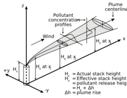
Visualization of a buoyant also known as Gaussian air pollutant dispersion plume
Air quality forecasting attempts to predict when the concentrations of pollutants will attain levels that are hazardous to public health. The concentration of pollutants in the atmosphere is determined by transport, diffusion, chemical transformation, and ground deposition.[8] Alongside pollutant source and terrain information, these models require data about the state of the fluid flow in the atmosphere to determine its transport and diffusion.[9] Within air quality models, parameterizations take into account atmospheric emissions from multiple relatively tiny sources (e.g. roads, fields, factories) within specific grid boxes.[10]
Problems with increased resolution
As model resolution increases, errors associated with moist convective processes are increased as assumptions which are statistically valid for larger grid boxes become questionable once the grid boxes shrink in scale towards the size of the convection itself. At resolutions greater than T639, which has a grid box dimension of about 30 kilometres (19 mi),[11] the Arakawa-Schubert convective scheme produces minimal convective precipitation, making most precipitation unrealistically stratiform in nature.[12]
Calibration
When a physical process is parameterized, two choices have to be made: what is the structural form (for instance, two variables can be related linearly) and what is the exact value of the parameters (for instance, the constant of proportionality). The process of determining the exact values of the parameters in a parameterization is called calibration, or sometimes less precise, tuning. Calibration is a difficult process, and different strategies are used to do it. One popular method is to run a model, or a submodel, and compare it to a small set of selected metrics, such as temperature. The parameters that lead to the model run which resembles reality best are chosen.[13]
See also
References
- ↑ Lu, Chunsong; Liu, Yangang; Niu, Shengjie; Krueger, Steven; Wagner, Timothy (2013). "Exploring parameterization for turbulent entrainment-mixing processes in clouds". Journal of Geophysical Research: Atmospheres 118: 185–194. doi:10.1029/2012JD018464.
- ↑ Narita, Masami; Shiro Ohmori (2007-08-06). "3.7 Improving Precipitation Forecasts by the Operational Nonhydrostatic Mesoscale Model with the Kain-Fritsch Convective Parameterization and Cloud Microphysics". 12th Conference on Mesoscale Processes. http://ams.confex.com/ams/pdfpapers/126017.pdf. Retrieved 2011-02-15.
- ↑ Frierson, Dargan (2000-09-14). "The Diagnostic Cloud Parameterization Scheme". University of Washington. pp. 4–5. http://www.atmos.washington.edu/~dargan/591/diag_cloud.tech.pdf.
- ↑ 4.0 4.1 McGuffie, K.; A. Henderson-Sellers (2005). A climate modelling primer. John Wiley and Sons. pp. 187–188. ISBN 978-0-470-85751-9.
- ↑ Stensrud, David J. (2007). Parameterization schemes: keys to understanding numerical weather prediction models. Cambridge University Press. p. 6. ISBN 978-0-521-86540-1. https://books.google.com/books?id=lMXSpRwKNO8C&q=radiation+mountain+parameterization+book&pg=PA56. Retrieved 2011-02-15.
- ↑ Melʹnikova, Irina N.; Alexander V. Vasilyev (2005). Short-wave solar radiation in the earth's atmosphere: calculation, observation, interpretation. Springer. pp. 226–228. ISBN 978-3-540-21452-6. https://books.google.com/books?id=vdg5BgBmMkQC&q=radiation+parameterization+book&pg=PA226.
- ↑ Stensrud, David J. (2007). Parameterization schemes: keys to understanding numerical weather prediction models. Cambridge University Press. pp. 12–14. ISBN 978-0-521-86540-1. https://books.google.com/books?id=lMXSpRwKNO8C&q=radiation+mountain+parameterization+book&pg=PA56. Retrieved 2011-02-15.
- ↑ Daly, Aaron; Paolo Zannetti (2007). "Chapter 2: Air Pollution Modeling – An Overview". Ambient Air Pollution. The Arab School for Science and Technology and The EnviroComp Institute. p. 16. http://www.envirocomp.org/books/chapters/2aap.pdf. Retrieved 2011-02-24.
- ↑ Baklanov, Alexander; Rasmussen, Alix; Fay, Barbara; Berge, Erik; Finardi, Sandro (September 2002). "Potential and Shortcomings of Numerical Weather Prediction Models in Providing Meteorological Data for Urban Air Pollution Forecasting". Water, Air, & Soil Pollution: Focus 2 (5): 43–60. doi:10.1023/A:1021394126149.
- ↑ Baklanov, Alexander; Grimmond, Sue; Mahura, Alexander (2009). Meteorological and Air Quality Models for Urban Areas. Springer. pp. 11–12. ISBN 978-3-642-00297-7. https://books.google.com/books?id=wh-Xf0WZQlMC&q=model+parameterization+air+quality+book&pg=PA11. Retrieved 2011-02-24.
- ↑ Hamill, Thomas M.; Whitaker, Jeffrey S.; Fiorino, Michael; Koch, Steven E.; Lord, Stephen J. (2010-07-19). "Increasing NOAA's computational capacity to improve global forecast modeling". National Oceanic and Atmospheric Administration. p. 9. http://www.esrl.noaa.gov/psd/people/tom.hamill/global_HPC_whitepaper_hamilletal.pdf.
- ↑ Hamilton, Kevin; Wataru Ohfuchi (2008). High resolution numerical modelling of the atmosphere and ocean. Springer. p. 17. ISBN 978-0-387-36671-5. https://books.google.com/books?id=yHQYWxHJqzgC&q=unstable+grid+box+convection&pg=PA17. Retrieved 2011-02-15.
- ↑ Hourdin, Frédéric; Mauritsen, Thorsten; Gettelman, Andrew; Golaz, Jean-Christophe; Balaji, Venkatramani; Duan, Qingyun; Folini, Doris; Ji, Duoying et al. (2016). "The Art and Science of Climate Model Tuning". Bulletin of the American Meteorological Society 98 (3): 589–602. doi:10.1175/BAMS-D-15-00135.1. ISSN 0003-0007.
Further reading
Plant, Robert S; Yano, Jun-Ichi (2015). Parameterization of Atmospheric Convection. Imperial College Press. ISBN 978-1-78326-690-6.
Atmospheric, oceanographic, cryospheric, and climate models |
|---|
|
Specific models |
|---|
| Climate | |
|---|
| Global weather | |
|---|
| Regional and mesoscale atmospheric | |
|---|
| Regional and mesoscale oceanographic | |
|---|
| Atmospheric dispersion | |
|---|
| Chemical transport | |
|---|
| Land surface parametrization | |
|---|
| Cryospheric models | |
|---|
| Discontinued | |
|---|
|
|
|
|
|---|
|
|
|
|
|---|
| Physical | |
|---|
| Flora and fauna | |
|---|
| Society | |
|---|
| By country | |
|---|
|
|
Society and climate change |
|---|
|
|
|
|---|
| General | |
|---|
| International | |
|---|
| Regional policy | |
|---|
| Protest | |
|---|
|
|
|
|
Background and theory |
|---|
| Measurements | |
|---|
| Theory | |
|---|
| Research | |
|---|
|
|
|

.svg)


