AA tree
An AA tree in computer science is a form of balanced tree used for storing and retrieving ordered data efficiently. AA trees are named after their originator, Swedish computer scientist Arne Andersson.[1]
AA trees are a variation of the red–black tree, a form of binary search tree which supports efficient addition and deletion of entries. Unlike red–black trees, red nodes on an AA tree can only be added as a right subchild. In other words, no red node can be a left sub-child. This results in the simulation of a 2–3 tree instead of a 2–3–4 tree, which greatly simplifies the maintenance operations. The maintenance algorithms for a red–black tree need to consider seven different shapes to properly balance the tree:
An AA tree on the other hand only needs to consider two shapes due to the strict requirement that only right links can be red:
Balancing rotations
Whereas red–black trees require one bit of balancing metadata per node (the color), AA trees require O(log(log(N))) bits of metadata per node, in the form of an integer "level". The following invariants hold for AA trees:
- The level of every leaf node is one.
- The level of every left child is exactly one less than that of its parent.
- The level of every right child is equal to or one less than that of its parent.
- The level of every right grandchild is strictly less than that of its grandparent.
- Every node of level greater than one has two children.
A link where the child's level is equal to that of its parent is called a horizontal link, and is analogous to a red link in the red–black tree. Individual right horizontal links are allowed, but consecutive ones are forbidden; all left horizontal links are forbidden. These are more restrictive constraints than the analogous ones on red–black trees, with the result that re-balancing an AA tree is procedurally much simpler than re-balancing a red–black tree.
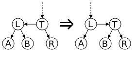
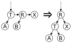
Insertions and deletions may transiently cause an AA tree to become unbalanced (that is, to violate the AA tree invariants). Only two distinct operations are needed for restoring balance: "skew" and "split". Skew is a right rotation to replace a subtree containing a left horizontal link with one containing a right horizontal link instead. Split is a left rotation and level increase to replace a subtree containing two or more consecutive right horizontal links with one containing two fewer consecutive right horizontal links. Implementation of balance-preserving insertion and deletion is simplified by relying on the skew and split operations to modify the tree only if needed, instead of making their callers decide whether to skew or split.
function skew is
    input: T, a node representing an AA tree that needs to be rebalanced.
    output: Another node representing the rebalanced AA tree.

    if nil(T) then
        return Nil
    else if nil(left(T)) then
        return T
    else if level(left(T)) == level(T) then
        Swap the pointers of horizontal left links.
        L = left(T)
        left(T) := right(L)
        right(L) := T
        return L
    else
        return T
    end if
end function
function split is
    input: T, a node representing an AA tree that needs to be rebalanced.
    output: Another node representing the rebalanced AA tree.

    if nil(T) then
        return Nil
    else if nil(right(T)) or  nil(right(right(T))) then
        return T
    else if level(T) == level(right(right(T))) then
        We have two horizontal right links.  Take the middle node, elevate it, and return it.
        R = right(T)
        right(T) := left(R)
        left(R) := T
        level(R) := level(R) + 1
        return R
    else
        return T
    end if
end function
Insertion
Insertion begins with the normal binary tree search and insertion procedure. Then, as the call stack unwinds (assuming a recursive implementation of the search), it's easy to check the validity of the tree and perform any rotations as necessary. If a horizontal left link arises, a skew will be performed, and if two horizontal right links arise, a split will be performed, possibly incrementing the level of the new root node of the current subtree. Note, in the code as given above, the increment of level(T). This makes it necessary to continue checking the validity of the tree as the modifications bubble up from the leaves.
function insert is
    input: X, the value to be inserted, and T, the root of the tree to insert it into.
    output: A balanced version T including X.

    Do the normal binary tree insertion procedure. Set the result of the
    recursive call to the correct child in case a new node was created or the
    root of the subtree changes.
    if nil(T) then
        Create a new leaf node with X.
        return node(X, 1, Nil, Nil)
    else if X < value(T) then
        left(T) := insert(X, left(T))
    else if X > value(T) then
        right(T) := insert(X, right(T))
    end if
    Note that the case of X == value(T) is unspecified. As given, an insert
    will have no effect. The implementor may desire different behavior.

    Perform skew and then split. The conditionals that determine whether or
    not a rotation will occur or not are inside of the procedures, as given
    above.
    T := skew(T)
    T := split(T)

    return T
end function
Deletion
As in most balanced binary trees, the deletion of an internal node can be turned into the deletion of a leaf node by swapping the internal node with either its closest predecessor or successor, depending on which are in the tree or on the implementor's whims. Retrieving a predecessor is simply a matter of following one left link and then all of the remaining right links. Similarly, the successor can be found by going right once and left until a null pointer is found. Because of the AA property of all nodes of level greater than one having two children, the successor or predecessor node will be in level 1, making their removal trivial.
To re-balance a tree, there are a few approaches. The one described by Andersson in his original paper is the simplest, and it is described here, although actual implementations may opt for a more optimized approach. After a removal, the first step to maintaining tree validity is to lower the level of any nodes whose children are two levels below them, or who are missing children. Then, the entire level must be skewed and split. This approach was favored, because when laid down conceptually, it has three easily understood separate steps:
- Decrease the level, if appropriate.
- Skew the level.
- Split the level.
However, we have to skew and split the entire level this time instead of just a node, complicating our code.
function delete is
    input: X, the value to delete, and T, the root of the tree from which it should be deleted.
    output: T, balanced, without the value X.

    if nil(T) then
        return T
    else if X > value(T) then
        right(T) := delete(X, right(T))
    else if X < value(T) then
        left(T) := delete(X, left(T))
    else
        If we're a leaf, easy, otherwise reduce to leaf case.
        if leaf(T) then
            return right(T)
        else if nil(left(T)) then
            L := successor(T)
            right(T) := delete(value(L), right(T))
            value(T) := value(L)
        else
            L := predecessor(T)
            left(T) := delete(value(L), left(T))
            value(T) := value(L)
        end if
    end if

    Rebalance the tree. Decrease the level of all nodes in this level if
    necessary, and then skew and split all nodes in the new level.
    T := decrease_level(T)
    T := skew(T)
    right(T) := skew(right(T))
    if not nil(right(T))
        right(right(T)) := skew(right(right(T)))
    end if
    T := split(T)
    right(T) := split(right(T))
    return T
end function
function decrease_level is
    input: T, a tree for which we want to remove links that skip levels.
    output: T with its level decreased.

    should_be = min(level(left(T)), level(right(T))) + 1
    if should_be < level(T) then
        level(T) := should_be
        if should_be < level(right(T)) then
            level(right(T)) := should_be
        end if
    end if
    return T
end function
A good example of deletion by this algorithm is present in the Andersson paper.
Performance
The performance of an AA tree is equivalent to the performance of a red–black tree. While an AA tree makes more rotations than a red–black tree, the simpler algorithms tend to be faster, and all of this balances out to result in similar performance. A red–black tree is more consistent in its performance than an AA tree, but an AA tree tends to be flatter, which results in slightly faster search times.[2]
See also
References
- ↑ Andersson, Arne (1993). "Balanced Search Trees made Simple". WADS '93: Proceedings of the Third Workshop on Algorithms and Data Structures (Springer-Verlag): 60-71. ISBN 3540571558.
- ↑ "A Disquisition on The Performance Behavior of Binary Search Tree Data Structures (pages 67-75)". http://www.cepis.org/upgrade/files/full-2004-V.pdf.
External links
- A. Andersson. Balanced search trees made simple
- A. Andersson. A note on searching in a binary search tree
- BSTlib – an open source AA tree library for C by trijezdci
- AA Visual 2007 1.5 - OpenSource Delphi program for educating AA tree structures
- Thorough tutorial Julienne Walker with lots of code, including a practical implementation
- Object Oriented implementation with tests
- A Disquisition on The Performance Behavior of Binary Search Tree Data Structures (pages 67–75) – comparison of AA trees, red–black trees, treaps, skip lists, and radix trees
- An Objective-C implementation
- Python implementation
 |


