Difference bound matrix
In model checking, a field of computer science, a difference bound matrix (DBM) is a data structure used to represent some convex polytopes called zones. This structure can be used to efficiently implement some geometrical operations over zones, such as testing emptiness, inclusion, equality, and computing the intersection and the sum of two zones. It is, for example, used in the Uppaal model checker; where it is also distributed as an independent library.[1]
More precisely, there is a notion of canonical DBM; there is a one-to-one relation between canonical DBMs and zones and from each DBM a canonical equivalent DBM can be efficiently computed. Thus, equality of zone can be tested by checking for equality of canonical DBMs.
Zone
A difference bound matrix is used to represents some kind of convex polytopes. Those polytopes are called zone. They are now defined. Formally, a zone is defined by equations of the form , , and , with and some variables, and a constant.
Zones have originally be called region,[2] but nowadays this name usually denote region, a special kind of zone. Intuitively, a region can be considered as a minimal non-empty zones, in which the constants used in constraint are bounded.
Given variables, there are exactly different non-redundant constraints possible, constraints which use a single variable and an upper bound, constraints which uses a single variable and a lower bound, and for each of the ordered pairs of variable , an upper bound on . However, an arbitrary convex polytope in may require an arbitrarily great number of constraints. Even when , there can be an arbitrary great number of non-redundant constraints , for some constants. This is the reason why DBMs can not be extended from zones to convex polytopes.
Example
As stated in the introduction, we consider a zone defined by a set of statements of the form , , and , with and some variables, and a constant. However some of those constraints are either contradictory or redundant. We now give such examples.
- the constraints and are contradictory. Hence, when two such constraints are found, the zone defined is empty.
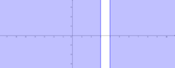
Figure in showing , which are disjoint - the constraints and are redundant. The second constraint being implied by the first one. Hence, when two such constraints are found in the definition of the zone, the second constraint may be removed.
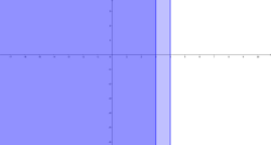
Figure in showing and which contains the first figure


We also give example showing how to generate new constraints from existing constraints. For each pair of clocks and , the DBM has a constraint of the form , where is either < or ≤. If no such constraint can be found, the constraint can be added to the zone definition without loss of generality. But in some case, a more precise constraint can be found. Such an example is now going to be given.
- the constraints , implies that . Thus, assuming that no other constraint such as or belongs to the definition, the constraint is added to the zone definition.
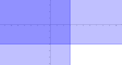
Figure in showing , and their intersections - the constraints , implies that . Thus, assuming that no other constraint such as or belongs to the definition, the constraint is added to the zone definition.
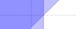
Figure in showing , and their intersections - the constraints , implies that . Thus, assuming that no other constraint such as or belongs to the definition, the constraint is added to the zone definition.
-3.png)

Actually, the two first cases above are particular cases of the third cases. Indeed, and can be rewritten as and respectively. And thus, the constraint added in the first example is similar to the constraint added in the third example.
Definition
We now fix a monoid which is a subset of the real line. This monoid is traditionally the set of integers, rationals, reals, or their subset of non-negative numbers.
Constraints
In order to define the data structure difference bound matrix, it is first required to give a data structure to encode atomic constraints. Furthermore, we introduce an algebra for atomic constraints. This algebra is similar to the tropical semiring, with two modifications:
- An arbitrary ordered monoid may be used instead of .
- In order to distinguish between "" and "", the set of elements of the algebra must contain information stating whether the order is strict or not.
Definition of constraints
The set of satisfiable constraints is defined as the set of pairs of the form:
- , with , which represents a constraint of the form ,
- , with , where is not a minimal element of , which represents a constraint of the form ,
- , which represents the absence of constraint.
The set of constraint contains all satisfiable constraints and contains also the following unsatisfiable constraint:
- .
The subset can not be defined using this kind of constraints. More generally, some convex polytopes can not be defined when the ordered monoid does not have the least-upper-bound property, even if each of the constraints in its definition uses at most two variables.
Operation on constraints
In order to generate a single constraint from a pair of constraints applied to the same (pair of) variable, we formalize the notion of intersection of constraints and of order over constraints. Similarly, in order to define a new constraints from existing constraints, a notion of sum of constraint must also be defined.
Order on constraints
We now define an order relation over constraints. This order symbolize the inclusion relation.
First, the set is considered as an ordered set, with < being inferior to ≤. Intuitively, this order is chosen because the set defined by is strictly included in the set defined by . We then state that the constraint is smaller than if either or ( and is less than ). That is, the order on constraints is the lexicographical order applied from right to left. Note that this order is a total order. If has the least-upper-bound property (or greatest-lower-bound property) then the set of constraints also have it.
Intersection of constraints
The intersection of two constraints, denoted as , is then simply defined as the minimum of those two constraints. If has the greatest-lower bound property then the intersection of an infinite number of constraints is also defined.
Sum of constraints
Given two variables and to which are applied constraints and , we now explain how to generate the constraint satisfied by . This constraint is called the sum of the two above-mentioned constraint, is denoted as and is defined as .
Constraints as an algebra
Here is a list of algebraic properties satisfied by the set of constraints.
- Both operations are associative and commutative,
- Sum is distributive over intersection, that is, for any three constraints, equals ,
- The intersection operation is idempotent,
- The constraint is an identity for the intersection operation,
- The constraint is an identity for the sum operation,
Furthermore, the following algebraic properties holds over satisfiable constraints:
- The constraint is a zero for the sum operation,
- It follows that the set of satisfiable constraints is an idempotent semiring, with as zero and as unity.
- If 0 is the minimum element of , then is a zero for the intersection constraints over satisfiable constraints.
Over non-satisfiable constraints both operations have the same zero, which is . Thus, the set of constraints does not even form a semiring, because the identity of the intersection is distinct from the zero of the sum.
DBMs
Given a set of variables, , a DBM is a matrix with column and rows indexed by and the entries are constraints. Intuitively, for a column and a row , the value at position represents . Thus, the zone defined by a matrix , denoted by , is .
Note that is equivalent to , thus the entry is still essentially an upper bound. Note however that, since we consider a monoid , for some values of and the real does not actually belong to the monoid.
Before introducing the definition of a canonical DBM, we need to define and discuss an order relation on those matrices.
Order on those matrices
A matrix is considered to be smaller than a matrix if each of its entries are smaller. Note that this order is not total. Given two DBMs and , if is smaller than or equal to , then .
The greatest-lower-bound of two matrices and , denoted by , has as its entry the value . Note that since is the «sum» operation of the semiring of constraints, the operation is the «sum» of two DBMs where the set of DBMs is considered as a module.
Similarly to the case of constraints, considered in section "Operation on constraints" above, the greatest-lower-bound of an infinite number of matrices is correctly defined as soon as satisfies the greatest-lower-bound property.
The intersection of matrices/zones is defined. The union operation is not defined, and indeed, a union of zone is not a zone in general.
For an arbitrary set of matrices which all defines the same zone , also defines . It thus follow that, as long as has the greatest-lower-bound property, each zone which is defined by at least a matrix has a unique minimal matrix defining it. This matrix is called the canonical DBM of .
First definition of canonical DBM
We restate the definition of a canonical difference bound matrix. It is a DBM such that no smaller matrix defines the same set. It is explained below how to check whether a matrix is a DBM, and otherwise how to compute a DBM from an arbitrary matrix such that both matrices represents the same set. But first, we give some examples.
Examples of matrices
We first consider the case where there is a single clock .
The real line
We first give the canonical DBM for . We then introduce another DBM which encode the set . This allow to find constraints which must be satisfied by any DBM.
The canonical DBM of the set of real is . It represents the constraints , , and . All of those constraints are satisfied independently of the value assigned to . In the remaining of the discussion, we will not explicitly describe constraints due to entries of the form , since those constraints are systematically satisfied.
The DBM also encodes the set of real. It contains the constraints and which are satisfied independently on the value of . This show that in a canonical DBM , a diagonal entry is never greater than , because the matrix obtained from by replacing the diagonal entry by defines the same set and is smaller than .
The empty set
We now consider many matrices which all encodes the empty set. We first give the canonical DBM for the empty set. We then explain why each of the DBM encodes the empty set. This allow to find constraints which must be satisfied by any DBM.
The canonical DBM of the empty set, over one variable, is . Indeed, it represents the set satisfying the constraint , , and . Those constraints are unsatisfiable.
The DBM also encodes the empty set. Indeed, it contains the constraint which is unsatisfiable. More generally, this show that no entry can be unless all entries are .
The DBM also encodes the empty set. Indeed, it contains the constraint which is unsatisfiable. More generally, this show that the entry in the diagonal line can not be smaller than unless it is .
The DBM also encodes the empty set. Indeed, it contains the constraints and which are contradictory. More generally, this show that, for each , if , then and are both equal to ≤.
The DBM also encodes the empty set. Indeed, it contains the constraints and which are contradictory. More generally, this show that for each , , unless is .
Strict constraints
The examples given in this section are similar to the examples given in the Example section above. This time, they are given as DBM.
The DBM represents the set satisfying the constraints and . As mentioned in the Example section, both of those constraints implies that . It means that the DBM encodes the same zone. Actually, it is the DBM of this zone. This shows that in any DBM , for each , the constraint is smaller than the constraint .
As explained in the Example section, the constant 0 can be considered as any variable, which leads to the more general rule: in any DBM , for each , the constraint is smaller than the constraint .
Three definition of canonical DBM
As explained in the introduction of the section Difference Bound Matrix, a canonical DBM is a DBM whose rows and columns are indexed by , whose entries are constraints. Furthermore, it follows one of the following equivalent properties.
- there are no smaller DBM defining the same zone,
- for each , the constraint is smaller than the constraint
- given the directed graph with edges and arrows labelled by , the shortest path from any edge to any edge is the arrow . This graph is called the potential graph of the DBM.
The last definition can be directly used to compute the canonical DBM associated to a DBM. It suffices to apply the Floyd–Warshall algorithm to the graph and associates to each entry the shortest path from to in the graph. If this algorithm detects a cycle of negative length, this means that the constraints are not satisfiable, and thus that the zone is empty.
Operations on zones
As stated in the introduction, the main interest of DBMs is that they allow to easily and efficiently implements operations on zones.
We first recall operations which were considered above:
- testing for the inclusion of a zone in a zone is done by testing whether the canonical DBM of is smaller than or equal to the DBM of ,
- A DBM for the intersection of a set of zones is the greatest-lower-bound of the DBM of those zones,
- testing for zone emptiness consists in checking whether the canonical DBM of the zone consists only of ,
- testing whether a zone is the entire space consists in checking whether the DBM of the zone consists only of .
We now describe operations which were not considered above. The first operations described below have clear geometrical meaning. The last ones become corresponds to operations which are more natural for clock valuations.
Sum of zones
The Minkowski sum of two zones, defined by two DBMs and , is defined by the DBM whose entry is . Note that since is the «product» operation of the semiring of constraints, the operation over DBMs is not actually an operation of the module of DBM.
In particular, it follows that, in order to translate a zone by a direction , it suffices to add the DBM of to the DBM of .
Projection of a component to a fixed value
Let a constant.
Given a vector , and an index , the projection of the -th component of to is the vector . In the language of clock, for , this corresponds to resetting the -th clock.
Projecting the -th component of a zone to consists simply in the set of vectors of with their -th component to . This is implemented on DBM by setting the components to and the components to
Future and past of a zone
Let us call the future the zone and the past the zone . Given a point , the future of is defined as , and the past of is defined as .
The names future and past comes from the notion of clock. If a set of clocks are assigned to the values , , etc. then in their future, the set of assignment they'll have is the future of .
Given a zone , the future of are the union of the future of each points of the zone. The definition of the past of a zone is similar. The future of a zone can thus be defined as , and hence can easily be implemented as a sum of DBMs. However, there is even a simpler algorithm to apply to DBM. It suffices to change every entries to . Similarly, the past of a zone can be computed by setting every entries to .
See also
- Region (model checking) – a zone, minimal under inclusion, satisfying some properties
References
- ↑ "UPPAAL DBM Library". 16 July 2021. https://github.com/UPPAALModelChecker/UDBM.
- ↑ Dill, David L (1990). "Timing assumptions and verification of finite-state concurrent systems". Automatic Verification Methods for Finite State Systems. Lecture Notes in Computer Science. 407. pp. 197–212. doi:10.1007/3-540-52148-8_17. ISBN 978-3-540-52148-8.
- Difference Bound Matrices Lecture #20 of Advanced Model Checking Joost-Pieter Katoen
- Péron, Mathias; Halbwachs, Nicolas (2008). "An Abstract Domain Extending Difference-Bound Matrices with Disequality Constraints". Verification, Model Checking, and Abstract Interpretation. Lecture Notes in Computer Science. 4349. pp. 268–282. doi:10.1007/978-3-540-69738-1_20. ISBN 978-3-540-69735-0. http://hal.archives-ouvertes.fr/docs/00/26/24/22/PDF/PeronHalbwachsVMCAI07.pdf.
 |  |
