Regression dilution

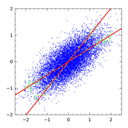
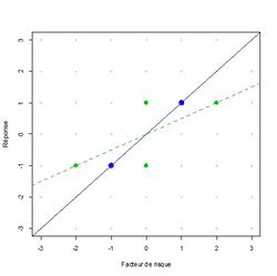
Regression dilution, also known as regression attenuation, is the biasing of the linear regression slope towards zero (the underestimation of its absolute value), caused by errors in the independent variable.
Consider fitting a straight line for the relationship of an outcome variable y to a predictor variable x, and estimating the slope of the line. Statistical variability, measurement error or random noise in the y variable causes uncertainty in the estimated slope, but not bias: on average, the procedure calculates the right slope. However, variability, measurement error or random noise in the x variable causes bias in the estimated slope (as well as imprecision). The greater the variance in the x measurement, the closer the estimated slope must approach zero instead of the true value.

It may seem counter-intuitive that noise in the predictor variable x induces a bias, but noise in the outcome variable y does not. Recall that linear regression is not symmetric: the line of best fit for predicting y from x (the usual linear regression) is not the same as the line of best fit for predicting x from y.[1]
Slope correction
Regression slope and other regression coefficients can be disattenuated as follows.
The case of a fixed x variable
The case that x is fixed, but measured with noise, is known as the functional model or functional relationship.[2] It can be corrected using total least squares[3] and errors-in-variables models in general.
The case of a randomly distributed x variable
The case that the x variable arises randomly is known as the structural model or structural relationship. For example, in a medical study patients are recruited as a sample from a population, and their characteristics such as blood pressure may be viewed as arising from a random sample.
Under certain assumptions (typically, normal distribution assumptions) there is a known ratio between the true slope, and the expected estimated slope. Frost and Thompson (2000) review several methods for estimating this ratio and hence correcting the estimated slope.[4] The term regression dilution ratio, although not defined in quite the same way by all authors, is used for this general approach, in which the usual linear regression is fitted, and then a correction applied. The reply to Frost & Thompson by Longford (2001) refers the reader to other methods, expanding the regression model to acknowledge the variability in the x variable, so that no bias arises.[5] Fuller (1987) is one of the standard references for assessing and correcting for regression dilution.[6]
Hughes (1993) shows that the regression dilution ratio methods apply approximately in survival models.[7] Rosner (1992) shows that the ratio methods apply approximately to logistic regression models.[8] Carroll et al. (1995) give more detail on regression dilution in nonlinear models, presenting the regression dilution ratio methods as the simplest case of regression calibration methods, in which additional covariates may also be incorporated.[9]
In general, methods for the structural model require some estimate of the variability of the x variable. This will require repeated measurements of the x variable in the same individuals, either in a sub-study of the main data set, or in a separate data set. Without this information it will not be possible to make a correction.
Multiple x variables
The case of multiple predictor variables subject to variability (possibly correlated) has been well-studied for linear regression, and for some non-linear regression models.[6][9] Other non-linear models, such as proportional hazards models for survival analysis, have been considered only with a single predictor subject to variability.[7]
Correlation correction
Charles Spearman developed in 1904 a procedure for correcting correlations for regression dilution,[10] i.e., to "rid a correlation coefficient from the weakening effect of measurement error".[11]
In measurement and statistics, the procedure is also called correlation disattenuation or the disattenuation of correlation.[12] The correction assures that the Pearson correlation coefficient across data units (for example, people) between two sets of variables is estimated in a manner that accounts for error contained within the measurement of those variables.[13]
Formulation
Let and be the true values of two attributes of some person or statistical unit. These values are variables by virtue of the assumption that they differ for different statistical units in the population. Let and be estimates of and derived either directly by observation-with-error or from application of a measurement model, such as the Rasch model. Also, let
where and are the measurement errors associated with the estimates and .
The estimated correlation between two sets of estimates is
which, assuming the errors are uncorrelated with each other and with the true attribute values, gives
where is the separation index of the set of estimates of , which is analogous to Cronbach's alpha; that is, in terms of classical test theory, is analogous to a reliability coefficient. Specifically, the separation index is given as follows:
where the mean squared standard error of person estimate gives an estimate of the variance of the errors, . The standard errors are normally produced as a by-product of the estimation process (see Rasch model estimation).
The disattenuated estimate of the correlation between the two sets of parameter estimates is therefore
That is, the disattenuated correlation estimate is obtained by dividing the correlation between the estimates by the geometric mean of the separation indices of the two sets of estimates. Expressed in terms of classical test theory, the correlation is divided by the geometric mean of the reliability coefficients of two tests.
Given two random variables and measured as and with measured correlation and a known reliability for each variable, and , the estimated correlation between and corrected for attenuation is
- .
How well the variables are measured affects the correlation of X and Y. The correction for attenuation tells one what the estimated correlation is expected to be if one could measure X′ and Y′ with perfect reliability.
Thus if and are taken to be imperfect measurements of underlying variables and with independent errors, then estimates the true correlation between and .
Applicability
A correction for regression dilution is necessary in statistical inference based on regression coefficients. However, in predictive modelling applications, correction is neither necessary nor appropriate. In change detection, correction is necessary.
To understand this, consider the measurement error as follows. Let y be the outcome variable, x be the true predictor variable, and w be an approximate observation of x. Frost and Thompson suggest, for example, that x may be the true, long-term blood pressure of a patient, and w may be the blood pressure observed on one particular clinic visit.[4] Regression dilution arises if we are interested in the relationship between y and x, but estimate the relationship between y and w. Because w is measured with variability, the slope of a regression line of y on w is less than the regression line of y on x. Standard methods can fit a regression of y on w without bias. There is bias only if we then use the regression of y on w as an approximation to the regression of y on x. In the example, assuming that blood pressure measurements are similarly variable in future patients, our regression line of y on w (observed blood pressure) gives unbiased predictions.
An example of a circumstance in which correction is desired is prediction of change. Suppose the change in x is known under some new circumstance: to estimate the likely change in an outcome variable y, the slope of the regression of y on x is needed, not y on w. This arises in epidemiology. To continue the example in which x denotes blood pressure, perhaps a large clinical trial has provided an estimate of the change in blood pressure under a new treatment; then the possible effect on y, under the new treatment, should be estimated from the slope in the regression of y on x.
Another circumstance is predictive modelling in which future observations are also variable, but not (in the phrase used above) "similarly variable". For example, if the current data set includes blood pressure measured with greater precision than is common in clinical practice. One specific example of this arose when developing a regression equation based on a clinical trial, in which blood pressure was the average of six measurements, for use in clinical practice, where blood pressure is usually a single measurement.[14]
All of these results can be shown mathematically, in the case of simple linear regression assuming normal distributions throughout (the framework of Frost & Thompson).
It has been discussed that a poorly executed correction for regression dilution, in particular when performed without checking for the underlying assumptions, may do more damage to an estimate than no correction.[15]
Further reading
Regression dilution was first mentioned, under the name attenuation, by Spearman (1904).[16] Those seeking a readable mathematical treatment might like to start with Frost and Thompson (2000).[4]
See also
- Errors-in-variables models
- Quantization (signal processing) – a common source of error in the explanatory or independent variables
References
- ↑ Draper, N.R.; Smith, H. (1998). Applied Regression Analysis (3rd ed.). John Wiley. pp. 19. ISBN 0-471-17082-8.
- ↑ Riggs, D. S. et al. (1978). "Fitting straight lines when both variables are subject to error". Life Sciences 22 (13–15): 1305–60. doi:10.1016/0024-3205(78)90098-x. PMID 661506.
- ↑ Golub, Gene H.; van Loan, Charles F. (1980). "An Analysis of the Total Least Squares Problem". SIAM Journal on Numerical Analysis (Society for Industrial & Applied Mathematics (SIAM)) 17 (6): 883–893. doi:10.1137/0717073. ISSN 0036-1429.
- ↑ 4.0 4.1 4.2 Frost, C. and S. Thompson (2000). "Correcting for regression dilution bias: comparison of methods for a single predictor variable." Journal of the Royal Statistical Society Series A 163: 173–190.
- ↑ Longford, N. T. (2001). "Correspondence". Journal of the Royal Statistical Society, Series A 164 (3): 565. doi:10.1111/1467-985x.00219.
- ↑ 6.0 6.1 Fuller, W. A. (1987). Measurement Error Models. New York: Wiley. ISBN 9780470317334. https://books.google.com/books?id=Nalc0DkAJRYC.
- ↑ 7.0 7.1 Hughes, M. D. (1993). "Regression dilution in the proportional hazards model". Biometrics 49 (4): 1056–1066. doi:10.2307/2532247. PMID 8117900.
- ↑ Rosner, B. et al. (1992). "Correction of Logistic Regression Relative Risk Estimates and Confidence Intervals for Random Within-Person Measurement Error". American Journal of Epidemiology 136 (11): 1400–1403. doi:10.1093/oxfordjournals.aje.a116453. PMID 1488967.
- ↑ 9.0 9.1 Carroll, R. J., Ruppert, D., and Stefanski, L. A. (1995). Measurement error in non-linear models. New York, Wiley.
- ↑ Spearman, C. (1904). "The Proof and Measurement of Association between Two Things". The American Journal of Psychology (University of Illinois Press) 15 (1): 72–101. doi:10.2307/1412159. ISSN 0002-9556. https://archive.org/download/proofmeasurement00speauoft/proofmeasurement00speauoft_bw.pdf. Retrieved 2021-07-10.
- ↑ Jensen, A.R. (1998). The g Factor: The Science of Mental Ability. Human evolution, behavior, and intelligence. Praeger. ISBN 978-0-275-96103-9.
- ↑ Osborne, Jason W. (2003-05-27). "Effect Sizes and the Disattenuation of Correlation and Regression Coefficients: Lessons from Educational Psychology". Practical Assessment, Research, and Evaluation 8 (1). doi:10.7275/0k9h-tq64. https://scholarworks.umass.edu/pare/vol8/iss1/11. Retrieved 2021-07-10.
- ↑ Franks, Alexander; Airoldi, Edoardo; Slavov, Nikolai (2017-05-08). "Post-transcriptional regulation across human tissues". PLOS Computational Biology 13 (5): e1005535. doi:10.1371/journal.pcbi.1005535. ISSN 1553-7358. PMID 28481885.
- ↑ Stevens, R. J.; Kothari, V.; Adler, A. I.; Stratton, I. M.; Holman, R. R. (2001). "Appendix to "The UKPDS Risk Engine: a model for the risk of coronary heart disease in type 2 diabetes UKPDS 56)". Clinical Science 101: 671–679. doi:10.1042/cs20000335.
- ↑ Davey Smith, G.; Phillips, A. N. (1996). "Inflation in epidemiology: 'The proof and measurement of association between two things' revisited". British Medical Journal 312 (7047): 1659–1661. doi:10.1136/bmj.312.7047.1659. PMID 8664725.
- ↑ Spearman, C (1904). "The proof and measurement of association between two things". American Journal of Psychology 15 (1): 72–101. doi:10.2307/1412159. https://archive.org/details/proofmeasurement00speauoft.
 |
