External ray

An external ray is a curve that runs from infinity toward a Julia or Mandelbrot set. Although this curve is only rarely a half-line (ray) it is called a ray because it is an image of a ray.

External rays are used in complex analysis, particularly in complex dynamics and geometric function theory.

History

External rays were introduced in Douady and Hubbard's study of the Mandelbrot set

Types

Criteria for classification :

• plane : parameter or dynamic
• map
• bifurcation of dynamic rays
• Stretching
• landing

plane

External rays of (connected) Julia sets on dynamical plane are often called dynamic rays.

External rays of the Mandelbrot set (and similar one-dimensional connectedness loci) on parameter plane are called parameter rays.

bifurcation

Dynamic ray can be:

• bifurcated = branched = broken
• smooth = unbranched = unbroken

When the filled Julia set is connected, there are no branching external rays. When the Julia set is not connected then some external rays branch.

stretching

Stretching rays were introduced by Branner and Hubbard:

"The notion of stretching rays is a generalization of that of external rays for the Mandelbrot set to higher degree polynomials."

landing

Every rational parameter ray of the Mandelbrot set lands at a single parameter.

Maps

Polynomials

Dynamical plane = z-plane

External rays are associated to a compact, full, connected subset [math]\displaystyle{ K\, }[/math] of the complex plane as :

• the images of radial rays under the Riemann map of the complement of [math]\displaystyle{ K\, }[/math]
• the gradient lines of the Green's function of [math]\displaystyle{ K\, }[/math]
• field lines of Douady-Hubbard potential
• an integral curve of the gradient vector field of the Green's function on neighborhood of infinity

External rays together with equipotential lines of Douady-Hubbard potential ( level sets) form a new polar coordinate system for exterior ( complement ) of [math]\displaystyle{ K\, }[/math].

In other words the external rays define vertical foliation which is orthogonal to horizontal foliation defined by the level sets of potential.

Uniformization

Let [math]\displaystyle{ \Psi_c\, }[/math] be the conformal isomorphism from the complement (exterior) of the closed unit disk [math]\displaystyle{ \overline{\mathbb{D}} }[/math] to the complement of the filled Julia set [math]\displaystyle{ \ K_c }[/math].

[math]\displaystyle{ \Psi_c: \hat{\Complex} \setminus \overline{\mathbb{D}} \to \hat{\Complex} \setminus K_c }[/math]

where [math]\displaystyle{ \hat{\Complex} }[/math] denotes the extended complex plane. Let [math]\displaystyle{ \Phi_c = \Psi_c^{-1}\, }[/math] denote the Boettcher map. [math]\displaystyle{ \Phi_c\, }[/math] is a uniformizing map of the basin of attraction of infinity, because it conjugates [math]\displaystyle{ f_c }[/math] on the complement of the filled Julia set [math]\displaystyle{ K_c }[/math] to [math]\displaystyle{ f_0(z)=z^2 }[/math] on the complement of the unit disk:

[math]\displaystyle{ \begin{align} \Phi_c: \hat{\Complex} \setminus K_c &\to \hat{\Complex} \setminus \overline{\mathbb{D}}\\ z & \mapsto \lim_{n\to \infty} (f_c^n(z))^{2^{-n}} \end{align} }[/math]

and

[math]\displaystyle{ \Phi_c \circ f_c \circ \Phi_c^{-1} = f_0 }[/math]

A value [math]\displaystyle{ w = \Phi_c(z) }[/math] is called the Boettcher coordinate for a point [math]\displaystyle{ z \in \hat{\Complex}\setminus K_c }[/math].

Formal definition of dynamic ray

Polar coordinate system and [math]\displaystyle{ \psi_c }[/math] for [math]\displaystyle{ c=-2 }[/math]

The external ray of angle [math]\displaystyle{ \theta\, }[/math] noted as [math]\displaystyle{ \mathcal{R}^K _{\theta} }[/math]is:

• the image under [math]\displaystyle{ \Psi_c\, }[/math] of straight lines [math]\displaystyle{ \mathcal{R}_{\theta} = \{\left(r\cdot e^{2\pi i \theta}\right) : \ r \gt 1 \} }[/math]

[math]\displaystyle{ \mathcal{R}^K _{\theta} = \Psi_c(\mathcal{R}_{\theta}) }[/math]

• set of points of exterior of filled-in Julia set with the same external angle [math]\displaystyle{ \theta }[/math]

[math]\displaystyle{ \mathcal{R}^K _{\theta} = \{ z\in \hat{\Complex} \setminus K_c : \arg(\Phi_c(z)) = \theta \} }[/math]

Properties

The external ray for a periodic angle [math]\displaystyle{ \theta\, }[/math] satisfies:

[math]\displaystyle{ f(\mathcal{R}^K _{\theta}) = \mathcal{R}^K _{2 \theta} }[/math]

and its landing point [math]\displaystyle{ \gamma_f(\theta) }[/math] satisfies:

[math]\displaystyle{ f(\gamma_f(\theta)) = \gamma_f(2\theta) }[/math]

Parameter plane = c-plane

"Parameter rays are simply the curves that run perpendicular to the equipotential curves of the M-set."

Uniformization

Boundary of Mandelbrot set as an image of unit circle under [math]\displaystyle{ \Psi_M\, }[/math]

Uniformization of complement (exterior) of Mandelbrot set

Let [math]\displaystyle{ \Psi_M\, }[/math] be the mapping from the complement (exterior) of the closed unit disk [math]\displaystyle{ \overline{\mathbb{D}} }[/math] to the complement of the Mandelbrot set [math]\displaystyle{ \ M }[/math].

[math]\displaystyle{ \Psi_M:\mathbb{\hat{C}}\setminus \overline{\mathbb{D}}\to\mathbb{\hat{C}}\setminus M }[/math]

and Boettcher map (function) [math]\displaystyle{ \Phi_M\, }[/math], which is uniformizing map of complement of Mandelbrot set, because it conjugates complement of the Mandelbrot set [math]\displaystyle{ \ M }[/math] and the complement (exterior) of the closed unit disk

[math]\displaystyle{ \Phi_M: \mathbb{\hat{C}}\setminus M \to \mathbb{\hat{C}}\setminus \overline{\mathbb{D}} }[/math]

it can be normalized so that :

[math]\displaystyle{ \frac{\Phi_M(c)}{c} \to 1 \ as\ c \to \infty \, }[/math]

where :

[math]\displaystyle{ \mathbb{\hat{C}} }[/math] denotes the extended complex plane

Jungreis function [math]\displaystyle{ \Psi_M\, }[/math] is the inverse of uniformizing map :

[math]\displaystyle{ \Psi_M = \Phi_{M}^{-1} \, }[/math]

In the case of complex quadratic polynomial one can compute this map using Laurent series about infinity

[math]\displaystyle{ c = \Psi_M (w) = w + \sum_{m=0}^{\infty} b_m w^{-m} = w -\frac{1}{2} + \frac{1}{8w} - \frac{1}{4w^2} + \frac{15}{128w^3} + ...\, }[/math]

where

[math]\displaystyle{ c \in \mathbb{\hat{C}}\setminus M }[/math]

[math]\displaystyle{ w \in \mathbb{\hat{C}}\setminus \overline{\mathbb{D}} }[/math]

Formal definition of parameter ray

The external ray of angle [math]\displaystyle{ \theta\, }[/math] is:

• the image under [math]\displaystyle{ \Psi_c\, }[/math] of straight lines [math]\displaystyle{ \mathcal{R}_{\theta} = \{\left(r*e^{2\pi i \theta}\right) : \ r \gt 1 \} }[/math]

[math]\displaystyle{ \mathcal{R}^M _{\theta} = \Psi_M(\mathcal{R}_{\theta}) }[/math]

• set of points of exterior of Mandelbrot set with the same external angle [math]\displaystyle{ \theta }[/math]

[math]\displaystyle{ \mathcal{R}^M _{\theta} = \{ c\in \mathbb{\hat{C}}\setminus M  : \arg(\Phi_M(c)) = \theta \} }[/math]

Definition of the Boettcher map

Douady and Hubbard define:

[math]\displaystyle{ \Phi_M(c) \ \overset{\underset{\mathrm{def}}{}}{=} \ \Phi_c(z=c)\, }[/math]

so external angle of point [math]\displaystyle{ c\, }[/math] of parameter plane is equal to external angle of point [math]\displaystyle{ z=c\, }[/math] of dynamical plane

External angle

• 

  collecting bits outwards

• 

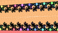
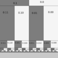  Binary decomposition of unrolled circle plane

• 

  binary decomposition of dynamic plane for f(z) = z^2

Angle θ is named external angle ( argument ).

Principal value of external angles are measured in turns modulo 1

1 turn = 360 degrees = 2 × π radians

Compare different types of angles :

• external ( point of set's exterior )
• internal ( point of component's interior )
• plain ( argument of complex number )

	external angle	internal angle	plain angle
parameter plane	[math]\displaystyle{ \arg(\Phi_M(c)) \, }[/math]	[math]\displaystyle{ \arg(\rho_n(c)) \, }[/math]	[math]\displaystyle{ \arg(c) \, }[/math]
dynamic plane	[math]\displaystyle{ \arg(\Phi_c(z)) \, }[/math]		[math]\displaystyle{ \arg(z) \, }[/math]

Computation of external argument

• argument of Böttcher coordinate as an external argument
  • [math]\displaystyle{ \arg_M(c) = \arg(\Phi_M(c)) }[/math]
  • [math]\displaystyle{ \arg_c(z) = \arg(\Phi_c(z)) }[/math]
• kneading sequence as a binary expansion of external argument

Transcendental maps

For transcendental maps ( for example exponential ) infinity is not a fixed point but an essential singularity and there is no Boettcher isomorphism.

Here dynamic ray is defined as a curve :

• connecting a point in an escaping set and infinity
• lying in an escaping set

Images

Dynamic rays

• unbranched
• 

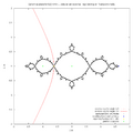  Julia set for [math]\displaystyle{ f_c(z) = z^2 -1 }[/math] with 2 external ray landing on repelling fixed point alpha

• 

  Julia set and 3 external rays landing on fixed point [math]\displaystyle{ \alpha_c\, }[/math]

• 

  Dynamic external rays landing on repelling period 3 cycle and 3 internal rays landing on fixed point [math]\displaystyle{ \alpha_c\, }[/math]

• 

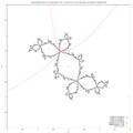
  Julia set with external rays landing on period 3 orbit

• 

  Rays landing on parabolic fixed point for periods 2-40

• branched
• 

  Branched dynamic ray

Parameter rays

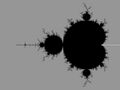
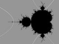
Mandelbrot set for complex quadratic polynomial with parameter rays of root points

• 

  External rays for angles of the form  : n / ( 2¹ - 1) (0/1; 1/1) landing on the point c= 1/4, which is cusp of main cardioid ( period 1 component)

• 

  External rays for angles of the form  : n / ( 2² - 1) (1/3, 2/3) landing on the point c= - 3/4, which is root point of period 2 component

• 

  External rays for angles of the form : n / ( 2³ - 1) (1/7,2/7) (3/7,4/7) landing on the point c= -1.75 = -7/4 (5/7,6/7) landing on the root points of period 3 components.

• 

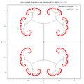
  External rays for angles of form  : n / ( 2⁴ - 1) (1/15,2/15) (3/15, 4/15) (6/15, 9/15) landing on the root point c= -5/4 (7/15, 8/15) (11/15,12/15) (13/15, 14/15) landing on the root points of period 4 components.

• 

  External rays for angles of form  : n / ( 2⁵ - 1) landing on the root points of period 5 components

• 

  internal ray of main cardioid of angle 1/3: starts from center of main cardioid c=0, ends in the root point of period 3 component, which is the landing point of parameter (external) rays of angles 1/7 and 2/7

• 

  Internal ray for angle 1/3 of main cardioid made by conformal map from unit circle

• 

  Mini Mandelbrot set with period 134 and 2 external rays

• 
• 
• 
• 

  Wakes near the period 3 island

• 

  Wakes along the main antenna

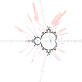
Parameter space of the complex exponential family f(z)=exp(z)+c. Eight parameter rays landing at this parameter are drawn in black.

Programs that can draw external rays

• Mandel - program by Wolf Jung written in C++ using Qt with source code available under the GNU General Public License
  • Java applets by Evgeny Demidov ( code of mndlbrot::turn function by Wolf Jung has been ported to Java ) with free source code
  • ezfract by Michael Sargent, uses the code by Wolf Jung
• OTIS by Tomoki KAWAHIRA - Java applet without source code
• Spider XView program by Yuval Fisher
• YABMP by Prof. Eugene Zaustinsky for DOS without source code
• DH_Drawer by Arnaud Chéritat written for Windows 95 without source code
• Linas Vepstas C programs for Linux console with source code
• Program Julia by Curtis T. McMullen written in C and Linux commands for C shell console with source code
• mjwinq program by Matjaz Erat written in delphi/windows without source code ( For the external rays it uses the methods from quad.c in julia.tar by Curtis T McMullen)
• RatioField by Gert Buschmann, for windows with Pascal source code for Dev-Pascal 1.9.2 (with Free Pascal compiler )
• Mandelbrot program by Milan Va, written in Delphi with source code
• Power MANDELZOOM by Robert Munafo
• ruff by Claude Heiland-Allen

See also

• external rays of Misiurewicz point
• Orbit portrait
• Periodic points of complex quadratic mappings
• Prouhet-Thue-Morse constant
• Carathéodory's theorem
• Field lines of Julia sets

References

• Lennart Carleson and Theodore W. Gamelin, Complex Dynamics, Springer 1993
• Adrien Douady and John H. Hubbard, Etude dynamique des polynômes complexes, Prépublications mathémathiques d'Orsay 2/4 (1984 / 1985)
• John W. Milnor, Periodic Orbits, External Rays and the Mandelbrot Set: An Expository Account; Géométrie complexe et systèmes dynamiques (Orsay, 1995), Astérisque No. 261 (2000), 277–333. (First appeared as a Stony Brook IMS Preprint in 1999, available as arXiV:math.DS/9905169.)
• John Milnor, Dynamics in One Complex Variable, Third Edition, Princeton University Press, 2006, ISBN:0-691-12488-4
• Wolf Jung : Homeomorphisms on Edges of the Mandelbrot Set. Ph.D. thesis of 2002

External links

• Hubbard Douady Potential, Field Lines by Inigo Quilez
• Intertwined Internal Rays in Julia Sets of Rational Maps by Robert L. Devaney
• Extending External Rays Throughout the Julia Sets of Rational Maps by Robert L. Devaney With Figen Cilingir and Elizabeth D. Russell
• John Hubbard's presentation, The Beauty and Complexity of the Mandelbrot Set, part 3.1
• videos by ImpoliteFruit
• Milan Va. "Mandelbrot set drawing". http://sweb.cz/milan_va/Mandelbrot/. Retrieved 2009-06-15.

References

- ↑ J. Kiwi : Rational rays and critical portraits of complex polynomials. Ph. D. Thesis SUNY at Stony Brook (1997); IMS Preprint #1997/15.
- ↑ Inou, Hiroyuki; Mukherjee, Sabyasachi (2016). "Non-landing parameter rays of the multicorns". Inventiones Mathematicae 204 (3): 869–893. doi:10.1007/s00222-015-0627-3. Bibcode: 2016InMat.204..869I.
- ↑ Atela, Pau (1992). "Bifurcations of dynamic rays in complex polynomials of degree two". Ergodic Theory and Dynamical Systems 12 (3): 401–423. doi:10.1017/S0143385700006854.
- ↑ Petersen, Carsten L.; Zakeri, Saeed (2020). "Periodic points and smooth rays". Conformal Geometry and Dynamics of the American Mathematical Society 25 (8): 170–178. doi:10.1090/ecgd/364.
- ↑ Holomorphic Dynamics: On Accumulation of Stretching Rays by Pia B.N. Willumsen, see page 12
- ↑ The iteration of cubic polynomials Part I : The global topology of parameter by BODIL BRANNER and JOHN H. HUBBARD
- ↑ Stretching rays for cubic polynomials by Pascale Roesch
- ↑ Komori, Yohei; Nakane, Shizuo (2004). "Landing property of stretching rays for real cubic polynomials". Conformal Geometry and Dynamics 8 (4): 87–114. doi:10.1090/s1088-4173-04-00102-x. Bibcode: 2004CGDAM...8...87K. https://www.ams.org/journals/ecgd/2004-08-04/S1088-4173-04-00102-X/S1088-4173-04-00102-X.pdf.
- ↑ A. Douady, J. Hubbard: Etude dynamique des polynˆomes complexes. Publications math´ematiques d’Orsay 84-02 (1984) (premi`ere partie) and 85-04 (1985) (deuxi`eme partie).
- ↑ Schleicher, Dierk (1997). "Rational parameter rays of the Mandelbrot set". arXiv:math/9711213.
- ↑ Video : The beauty and complexity of the Mandelbrot set by John Hubbard ( see part 3 )
- ↑ Yunping Jing : Local connectivity of the Mandelbrot set at certain infinitely renormalizable points Complex Dynamics and Related Topics, New Studies in Advanced Mathematics, 2004, The International Press, 236-264
- ↑ POLYNOMIAL BASINS OF INFINITY LAURA DEMARCO AND KEVIN M. PILGRIM
- ↑ How to draw external rays by Wolf Jung
- ↑ Tessellation and Lyubich-Minsky laminations associated with quadratic maps I: Pinching semiconjugacies Tomoki Kawahira[Usurped!]
- ↑ Douady Hubbard Parameter Rays by Linas Vepstas
- ↑ John H. Ewing, Glenn Schober, The area of the Mandelbrot Set
- ↑ Irwin Jungreis: The uniformization of the complement of the Mandelbrot set. Duke Math. J. Volume 52, Number 4 (1985), 935-938.
- ↑ Adrien Douady, John Hubbard, Etudes dynamique des polynomes complexes I & II, Publ. Math. Orsay. (1984-85) (The Orsay notes)
- ↑ Bielefeld, B.; Fisher, Y.; Vonhaeseler, F. (1993). "Computing the Laurent Series of the Map Ψ: C − D → C − M". Advances in Applied Mathematics 14: 25–38. doi:10.1006/aama.1993.1002.
- ↑ Weisstein, Eric W. "Mandelbrot Set." From MathWorld--A Wolfram Web Resource
- ↑ An algorithm to draw external rays of the Mandelbrot set by Tomoki Kawahira
- ↑ http://www.mrob.com/pub/muency/externalangle.html External angle at Mu-ENCY (the Encyclopedia of the Mandelbrot Set) by Robert Munafo
- ↑ Computation of the external argument by Wolf Jung
- ↑ A. DOUADY, Algorithms for computing angles in the Mandelbrot set (Chaotic Dynamics and Fractals, ed. Barnsley and Demko, Acad. Press, 1986, pp. 155-168).
- ↑ Adrien Douady, John H. Hubbard: Exploring the Mandelbrot set. The Orsay Notes. page 58
- ↑ Exploding the Dark Heart of Chaos by Chris King from Mathematics Department of University of Auckland
- ↑ Topological Dynamics of Entire Functions by Helena Mihaljevic-Brandt
- ↑ Dynamic rays of entire functions and their landing behaviour by Helena Mihaljevic-Brandt