Fractal flame


Fractal flames are a member of the iterated function system class[1] of fractals created by Scott Draves in 1992.[2] Draves' open-source code was later ported into Adobe After Effects graphics software[3] and translated into the Apophysis fractal flame editor.[2]
Fractal flames differ from ordinary iterated function systems in three ways:
- Nonlinear functions are iterated in addition to affine transforms.
- Log-density display instead of linear or binary (a form of tone mapping)
- Color by structure (i.e. by the recursive path taken) instead of monochrome or by density.
The tone mapping and coloring are designed to display as much of the detail of the fractal as possible, which generally results in a more aesthetically pleasing image.
Algorithm
The algorithm consists of two steps: creating a histogram and then rendering the histogram.
Creating the histogram

First, one iterates a set of functions, starting from a randomly chosen point P = (P.x,P.y,P.c), where the third coordinate indicates the current color of the point.
- Set of flame functions:
In each iteration, choose one of the functions above where the probability that Fj is chosen is pj. Then one computes the next iteration of P by applying Fj on (P.x,P.y).
Each individual function has the following form:
where the parameter wk is called the weight of the variation Vk. Draves suggests [4] that all :s are non-negative and sum to one, but implementations such as Apophysis do not impose that restriction.
The functions Vk are a set of predefined functions. A few examples[4] are
- V0(x,y) = (x,y) (Linear)
- V1(x,y) = (sin x,sin y) (Sinusoidal)
- V2(x,y) = (x,y)/(x2+y2) (Spherical)
The color P.c of the point is blended with the color associated with the latest applied function Fj:
- P.c := (P.c + (Fj)color) / 2
After each iteration, one updates the histogram at the point corresponding to (P.x,P.y). This is done as follows:
histogram[x][y][FREQUENCY] := histogram[x][y][FREQUENCY]+1
histogram[x][y][COLOR] := (histogram[x][y][COLOR] + P.c)/2
The colors in the image will therefore reflect what functions were used to get to that part of the image.
Rendering an image
To increase the quality of the image, one can use supersampling to decrease the noise. This involves creating a histogram larger than the image so each pixel has multiple data points to pull from. For example, create a histogram with 300×300 cells in order to draw a 100×100 px image; each pixel would use a 3×3 group of histogram buckets to calculate its value.
For each pixel (x,y) in the final image, do the following computations:
frequency_avg[x][y]  := average_of_histogram_cells_frequency(x,y);
color_avg[x][y] := average_of_histogram_cells_color(x,y);

alpha[x][y] := log(frequency_avg[x][y]) / log(frequency_max);
//frequency_max is the maximal number of iterations that hit a cell in the histogram.

final_pixel_color[x][y] := color_avg[x][y] * alpha[x][y]^(1/gamma); //gamma is a value greater than 1.
The algorithm above uses gamma correction to make the colors appear brighter. This is implemented in for example the Apophysis software.
To increase the quality even more, one can use gamma correction on each individual color channel, but this is a very heavy computation, since the log function is slow.
A simplified algorithm would be to let the brightness be linearly dependent on the frequency:
final_pixel_color[x][y] := color_avg[x][y] * frequency_avg[x][y]/frequency_max;
but this would make some parts of the fractal lose detail, which is undesirable.[4]
Density estimation
The flame algorithm is like a Monte Carlo simulation, with the flame quality directly proportional to the number of iterations of the simulation. The noise that results from this stochastic sampling can be reduced by blurring the image, to get a smoother result in less time. One does not however want to lose resolution in the parts of the image that receive many samples and so have little noise.
This problem can be solved with adaptive density estimation to increase image quality while keeping render times to a minimum. FLAM3 uses a simplification of the methods presented in *Adaptive Filtering for Progressive Monte Carlo Image Rendering*, a paper presented at WSCG 2000 by Frank Suykens and Yves D. Willems. The idea is to vary the width of the filter inversely proportional to the number of samples available.
As a result, areas with few samples and high noise become blurred and smoothed, but areas with many samples and low noise are left unaffected.[5]
Not all Flame implementations use density estimation.
See also
- Apophysis, an open source fractal flame editor for Microsoft Windows and Macintosh.
- Electric Sheep, a screen saver created by the inventor of fractal flames which renders and displays them through distributed computing.
- GIMP, a free software, multi OS image manipulation program that can generate fractal flames.
References
- ↑ Mitchell Whitelaw (2004). Metacreation: Art and Artificial Life. MIT Press. pp 155.
- ↑ 2.0 2.1 "Information about Apophysis software". http://apophysis.wikispaces.com/.
- ↑ Chris Gehman and Steve Reinke (2005). The Sharpest Point: Animation at the End of Cinema. YYZ Books. pp 269.
- ↑ 4.0 4.1 4.2 "The Fractal Flame Algorithm". https://flam3.com/flame_draves.pdf. (22.5 MB)
- ↑ See https://github.com/scottdraves/flam3/wiki/Density-Estimation.
| Open-source |  | ||||
|---|---|---|---|---|---|
| GNU | |||||
| Freeware | |||||
| Retail |
| ||||
| Scenery generator | |||||
| Found objects | |||||
| Related | |||||
| Characteristics |    | |
|---|---|---|
| Iterated function system | ||
| Strange attractor | ||
| L-system | ||
| Escape-time fractals | ||
| Rendering techniques | ||
| Random fractals | ||
| People | ||
| Other | ||
 |  |
