GenI process

The GenI process (/dʒiːnaɪ/ for Generic Intelligence) models team decision making by launching a chaotic competition between so-called ideas, where one idea after another dwindles out until exactly one remains. The decision statistics are completely determined by the process start configuration and match those known from quantum measurements. The random process accomplishes this in a natural way without any fine adjustment. Therefore, it is also of interest for the interpretation of physical processes. In mathematical terms, the GenI process describes a time-discrete stochastic process [math]\displaystyle{ X: [0,1] \times \mathbb{N}_0 \rightarrow 2^E }[/math] in the state space of the finite subsets of a countable set E, together with a mapping [math]\displaystyle{ 2^E \rightarrow \mathbb{C}^n }[/math] of the power set on E into an n-dimensional complex vector space. In principle, it can be classified as a Markov chain of first order, with variable transition probabilities [math]\displaystyle{ P(X_{n+1} \mid X_n) }[/math].

There are two expressions of the GenI process, for [math]\displaystyle{ n \geq 2 }[/math] and for [math]\displaystyle{ n=2 }[/math].

GenI process on eigenvector swarms

Background

The GenI random process determines changes in the complex vector space from the random behavior of independent individuals within a swarm-like construct. The swarm has a superposition state [math]\displaystyle{ \sum_{j=1}^n \beta_j e_j \in \mathbb{C}^n }[/math], that controls the individual activities via a target function. The amplitudes [math]\displaystyle{ \beta_j e_j }[/math] are also called ideas (cf "Generalized Quantum Modeling" ). The swarm takes one of the eigenstates [math]\displaystyle{ \gamma e_j }[/math] after a finite number of steps, with the well-defined probability [math]\displaystyle{ \frac {\vert{\beta_j}\vert^2} {\sum_k {\vert \beta_k \vert}^2} }[/math]. The individuals follow defined rules and are allowed to make mistakes, based on the processes in simulated shoals of fish. The GenI algorithm starts a chaotic decision-making process as a competition of ideas, such as running in a team that has to choose from a limited number of solutions to a given task. In the course of the process, a selection mechanism leads to ideas becoming extinct one after the other until finally just one survives that represents the solution to the problem.

Definition

Terminology

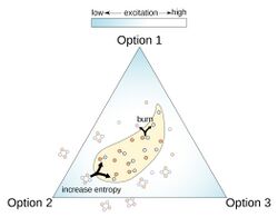
The GenI Process: A GenI swarm constantly sucks null rings from its environment and burns them randomly. The GenI process sets a gradient towards reducing the excitation. The swarm's state finally arrives at one of the given options.

Let E be a countable set and [math]\displaystyle{ \tilde E := \{ S \subset E : \vert S \vert \lt \infty \} \subset 2^E }[/math] the set of finite subsets of E. Next [math]\displaystyle{ B = (e_1, \ldots, e_n) }[/math] the canonical basis in [math]\displaystyle{ \mathbb{C}^n }[/math] and [math]\displaystyle{ \tilde B := \{i^k e_j : k = 0 \ldots 3, j = 1 \ldots n \} }[/math], where i is the imaginary unit in [math]\displaystyle{ \mathbb{C} }[/math].

A given [math]\displaystyle{ \rho : E \rightarrow \tilde B }[/math] maps each element of E into [math]\displaystyle{ \tilde B }[/math], so that [math]\displaystyle{ \forall e \in \tilde B : \vert \rho^{-1} (\{e\}) \vert = \infty }[/math]. For a set [math]\displaystyle{ S \in \tilde E }[/math] the complex vector [math]\displaystyle{ \rho(S) := \sum_{s \in S} \rho(s) = \sum_j \beta_j e_j }[/math] denotes its state with complex amplitudes [math]\displaystyle{ \beta_j }[/math]. Each such set S is called an Eigenvector-swarm or E-swarm.

A pair [math]\displaystyle{ s, t \in E }[/math] with [math]\displaystyle{ \rho(s) + \rho(t) = 0 }[/math] is a null pair. A tuple [math]\displaystyle{ (s_0, s_1, s_2, s_3) }[/math] is called a null ring generated by [math]\displaystyle{ s_0 }[/math], if [math]\displaystyle{ \exists j : \rho(s_k) = i^k e_j }[/math].

A set [math]\displaystyle{ N \in \tilde E }[/math] is called a null set, if [math]\displaystyle{ \rho(N) = 0 }[/math]. A maximal null set [math]\displaystyle{ N \subset S }[/math] is called the entropy of S and [math]\displaystyle{ S \setminus N }[/math] the entropy free residual swarm.

The term [math]\displaystyle{ \varepsilon_j (S) := 2 \frac {\vert \beta_j \vert \sqrt{\sum_{k \neq j} \vert \beta_k \vert^2}} {\sum_{k=1}^n \vert \beta_k\vert^2} \in [0; 1] }[/math] denotes the excitation of the swarm in index j.

Algorithm

Let [math]\displaystyle{ S^{(l)} = S_D^{(l)} + N_S^{(l)} }[/math] be a series of swarms (as an instantiation of [math]\displaystyle{ X(\omega, l) }[/math]) with the respective separation into a maximal null swarm [math]\displaystyle{ N_S^{(l)} }[/math] and the entropy free residual swarm [math]\displaystyle{ S_D^{(l)} }[/math], [math]\displaystyle{ \rho(S^{(l)}) =\sum_{k=1}^{n} \beta_k^{(l)} e_k }[/math] the respective state and [math]\displaystyle{ \varepsilon_j^{(l)} := \varepsilon_j(S^{(l)}) }[/math] the excitations.

1. Step: Set [math]\displaystyle{ l \leftarrow 0 }[/math] and start with a given swarm [math]\displaystyle{ S^{(0)} }[/math].
2. Step: If [math]\displaystyle{ \forall j : \varepsilon_j^{(l)} = 0 }[/math], then finish the process.
3. Step: Each element [math]\displaystyle{ s \in S_D^{(l)} }[/math] generates an additional null ring within the swarm.
4. Step: Each null pair [math]\displaystyle{ r,t \in N_S^{(l)} }[/math] (including the newly generated) with [math]\displaystyle{ \rho( r)= i^k e_j }[/math], [math]\displaystyle{ \rho( t)= - i^k e_j }[/math] gets selected with probability [math]\displaystyle{ p= \varepsilon_j^{(l) 2} }[/math] (and "burned" in the next step).
5. Step: For each selected null pair [math]\displaystyle{ r,t \in N_S^{(l)} }[/math], t leaves the swarm with probability [math]\displaystyle{ \frac {\varepsilon_j(S \setminus \{r\})} {\varepsilon_j(S \setminus \{r\}) + \varepsilon_j(S \setminus \{t\})} }[/math]. Otherwise t stays and r leaves the swarm.
6. Step: The resulting swarm is [math]\displaystyle{ S^{(l+1)} }[/math].
7. Step: Set [math]\displaystyle{ l \leftarrow l+1 }[/math] and start over with step 2.

Interpretation

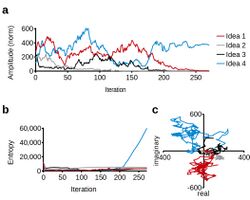
Competition of ideas within an GenI swarm: Graph a shows the evolution of absolute amplitudes during a GenI process operating in a four options environment. Due to its intrinsically chaotic behavior, it is impossible to predict the GenI process evolution at any point. The option with the lowest initial chance finally wins. Chart b shows the according evolution of entropy rising dramatically at the end for the winning idea. Figure c displays the native paths of each idea in the complex plane.

As soon as the excitation disappears in each index, the process naturally comes to rest in step 4 (except for the hard abort condition in step 2), since no null pair is "burned" and the state of the swarm no longer changes. The role of the excitation here reminds of the dynamics of a grain of sand in the formation of the Chladnic sound figures. On the other hand, excitation as a target in step 5 leads to a systematic distortion from 50% likelihood for an individual to remain. This leads here to an improved tendency to reduce the excitation. The following interpretation is obvious based on biological swarm behavior: Each individual tends to follow the rule "reduce the excitation". It remains free in its decision to do nothing (step 4), to follow the rule, or to disregard it (step 5).

Simulation

The reference implementation under JAVA shows an excellent convergence of the process. The table shows an example of the result of 1000 simulation runs (each simulation run aborts after more than 500 iterations or for swarm sizes> 10 million for performance reasons):

	[math]\displaystyle{ e_1 }[/math]	[math]\displaystyle{ e_2 }[/math]	[math]\displaystyle{ e_3 }[/math]	[math]\displaystyle{ e_4 }[/math]	[math]\displaystyle{ e_5 }[/math]	[math]\displaystyle{ e_6 }[/math]	[math]\displaystyle{ e_7 }[/math]	[math]\displaystyle{ e_8 }[/math]	[math]\displaystyle{ e_9 }[/math]	[math]\displaystyle{ e_{10} }[/math]
target	132	81	97	78	11	206	3	336	36	3
frequency	135	74	99	76	15	189	1	357	36	1
sigma	10.7	8.6	9.4	8.5	3.3	12.8	1.8	14.9	5.9	1.8
measurements scheduled			1000	of it divergent		17	convergent			983
statistics: chi square value: 7.85 ; chi critical value at 95% confidence: 16.9
medium swarm size: 300,418					sigma: 281,543		maximal: 1,008,512		minimal: 9,695

These results support the statement of convergence (hypothesis):

Let [math]\displaystyle{ S^{(0)} = S }[/math] be a given E-swarm with [math]\displaystyle{ \rho(S) = \sum_{j=1}^n \beta_j a_j }[/math], [math]\displaystyle{ n \ge 2 }[/math], [math]\displaystyle{ b_j = \vert \beta_j \vert }[/math], [math]\displaystyle{ \vert S \vert = \sqrt{\sum b_j^2} }[/math].

Let [math]\displaystyle{ S : \mathbb{N}_0 \times [0; 1] \rightarrow \tilde E }[/math] be a GenI process with [math]\displaystyle{ \rho ( S^{(m)}(\omega))=\sum \beta_j^{(m)}(\omega) a_j }[/math].

Then [math]\displaystyle{ P \left(\tilde S^{(m)} \underset{m \rightarrow \infty}\longrightarrow \gamma a_j \right) =P \left(\sum_{k \ne j} b_k^{(m) 2} \underset{m \rightarrow \infty}\longrightarrow 0 \right) = \frac{b_j^2}{\vert {S} \vert^2}. }[/math]

GenI process on Pauli swarms

The P(auli) process represents a special version of the GenI process for binary YES-NO decisions. It determines a time discrete stochastic process [math]\displaystyle{ X: [0;1] \times \mathbb{N}_0 \mapsto 2^E }[/math] in the state space of finite subsets of a countable set E, together with a map [math]\displaystyle{ \rho : 2^E \rightarrow \mathbb{C}^{2 \times 2} }[/math] from the power set on E into the complex matrix algebra [math]\displaystyle{ \mathbb{C}^{2 \times 2} }[/math], a perspective vector [math]\displaystyle{ v \in \mathbb{C}^2 }[/math] and a basis [math]\displaystyle{ a_1, a_2 \in \mathbb{C}^2 }[/math].

Background

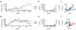
Competition within a GenI-swarm: The diagrams a-c demonstrate the Pauli process (as a special expression of the GenI process) evolution using a fixed perspective p = (1;1) under an external environment defined by the observable p3. Diagrams d-f show another test case under the internal environment defined by the swarm itself. Graphs a/d show the evolution of absolute amplitudes. Charts b/e show the according evolution of entropy for each type according to the swarm member images in {p0, ... , p3}. Null pairs for P-swarm do not relate to environment options as is true for E-swarms. Figures c/f display the native paths of each idea in the complex plane.

The GenI random process determines changes in the complex vector space out of the random behavior of independent individuals within a swarm-like construct. The swarm S has an image [math]\displaystyle{ \rho(S) \in \mathbb{C}^{2 \times 2} }[/math] in the complex matrix algebra. Together with a perspective [math]\displaystyle{ v \in \mathbb{C}^2 }[/math], the state of the swarm is determined by [math]\displaystyle{ \tilde S = \rho(S) v }[/math]. A basis [math]\displaystyle{ a_1, a_2 \in \mathbb{C}^2 }[/math] is called the environment and represents the options under which the swarm makes a decision. This can also be the eigenvectors of [math]\displaystyle{ \rho(S) \in \mathbb{C}^{2 \times 2} }[/math] itself and so create a self-reference. The environment, perspective and state of the swarm control the individual activities via a target variable (excitation). The amplitudes [math]\displaystyle{ \beta_j a_j }[/math] in the decomposition are also referred to as ideas with respect to the environment (see regarding "Generalized Quantum Modeling" ). The swarm takes one of the eigenstates [math]\displaystyle{ \gamma a_j }[/math] after a finite number of steps, with the well-defined probability [math]\displaystyle{ \frac {\vert{\beta_j}\vert^2} {{\vert \beta_1 \vert}^2 + {\vert \beta_2 \vert}^2} }[/math]. The individuals follow defined rules and are allowed to make mistakes, based on the processes in simulated shoals of fish. The GenI algorithm starts a chaotic decision-making process as a competition of ideas, such as running in a team that has two possible solutions to a given task. In the course of the process, a selection mechanism leads to the survival of only one of the two ideas that represents the solution to the problem. The model in principal allows a moving environment.

The special properties of the P-process also allow interpretations of physical processes (see in particular Carl Friedrich von Weizsäcker's ur-alternatives (archetypal objects), which he outlined for the reconstruction of quantum mechanics).

Definition

Terminology

Let E be a countable set and [math]\displaystyle{ \tilde E := \{ S \subset E : \vert S \vert \lt \infty \} \subset 2^E }[/math] the set of finite subsets of E. Next [math]\displaystyle{ P = (p_0, p_1, p_2, p_3) \subset \mathbb{C}^{2 \times 2} }[/math] the Pauli matrices and [math]\displaystyle{ \tilde P := \{i^k p_j : k = 0, \ldots, 3, j = 1, \ldots, n \} }[/math] the image of the Pauli group in the complex matrix algebra as its irreducible representation. Such a subset [math]\displaystyle{ S \in \tilde E }[/math] is called a Pauli-swarm or a P-swarm.

A given [math]\displaystyle{ \rho : E \rightarrow \tilde P }[/math] maps each element of E onto one element of the Pauli group, so that [math]\displaystyle{ \forall e \in \tilde P : \vert \rho^{-1} (\{e\}) \vert = \infty }[/math].

A basis [math]\displaystyle{ a_1, a_2 \in \mathbb{C}^2 }[/math] is called an environment, a non zero vector [math]\displaystyle{ v \in \mathbb{C}^2 }[/math] a perspective.

For a swarm [math]\displaystyle{ S \in \tilde E }[/math] denotes [math]\displaystyle{ \rho(S)  := \sum_{s \in S} \rho(s) }[/math] its matrix image, [math]\displaystyle{ \tilde S = \rho(S) v := \beta_1 a_1 + \beta_2 a_2 }[/math] its state with complex amplitudes [math]\displaystyle{ \beta_j }[/math] at the given environment and perspective.

A pair [math]\displaystyle{ s, t \in E }[/math] with [math]\displaystyle{ \rho(s) + \rho(t) = 0 }[/math] is a null pair. A tuple [math]\displaystyle{ (s_0, s_1, s_2, s_3) }[/math] is called a null ring generated by [math]\displaystyle{ s_0 }[/math], if [math]\displaystyle{ \exists j : \rho(s_k) = i^k p_j }[/math].

A set [math]\displaystyle{ N \in \tilde E }[/math] is called null set, if [math]\displaystyle{ \rho(N) = 0 }[/math]. A maximal null set [math]\displaystyle{ N \subset S }[/math] ist called the entropy of S and [math]\displaystyle{ S \setminus N }[/math] its entropy freed residual swarm.

The term [math]\displaystyle{ \varepsilon (S) := 2 \frac {\vert \beta_1 \vert \vert \beta_2 \vert} {\vert \beta_1\vert^2 + \vert \beta_2\vert^2} \in [0; 1] }[/math] denotes the excitation of the swarm.

Algorithm

Let [math]\displaystyle{ S^{(l)} = S_D^{(l)} + N_S^{(l)} }[/math] be a series of swarms (as an instance von [math]\displaystyle{ X(\omega, l) }[/math]) with the respective separation in a maximal null swarm [math]\displaystyle{ N_S^{(l)} }[/math] and the entropy freed residual swarm [math]\displaystyle{ S_D^{(l)} }[/math], [math]\displaystyle{ \tilde S^{(l)} =\beta_1^{(l)} a_1 + \beta_2^{(l)} a_2 }[/math] the respective states and [math]\displaystyle{ \varepsilon^{(l)} := \varepsilon(S^{(l)}) }[/math] the excitations.

1. Step: Set [math]\displaystyle{ l \leftarrow 0 }[/math] and start with a given swarm [math]\displaystyle{ S^{(0)} }[/math].
2. Step: If [math]\displaystyle{ \varepsilon^{(l)} = 0 }[/math], then finish the process.
3. Step: Each element [math]\displaystyle{ s \in S_D^{(l)} }[/math] generates an additional null ring within the swarm.
4. Step: Each null pair [math]\displaystyle{ r,t \in N_S^{(l)} }[/math] (including the newly generated) gets selected with probability [math]\displaystyle{ p= \varepsilon^{(l) 2} }[/math] (and gets "burned" in next step).
5. Step: For each selected null pair [math]\displaystyle{ r,t \in N_S^{(l)} }[/math], t leaves the swarm with probability [math]\displaystyle{ \frac {\varepsilon(S \setminus \{r\})} {\varepsilon(S \setminus \{r\}) + \varepsilon(S \setminus \{t\})} }[/math]. Otherwise t stays and r leaves the swarm.
6. Step: The resulting swarm is [math]\displaystyle{ S^{(l+1)} }[/math].
7. Step: Set [math]\displaystyle{ l \leftarrow l+1 }[/math] and start over with step 2.

Simulation

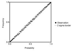
GenI swarms observations along target values from 0 to 1: The sample comprises 1000 measurements each on 201 test points on P(auli)-swarms (a special expression of a Geni swarm). More than 97% of observed frequencies are in the 2 sigma interval around the target values expected from quantum measurements. The chi square test value 92.6 is much lower than the critical level 168 at 95% confidence and 200 degrees of freedom.

The reference implementation under JAVA shows an excellent convergence of the process at any fixed environment and perspective according to the chart right hand.

The results support the statement of convergence (hypothesis):

Let [math]\displaystyle{ S^{(0)} = S }[/math] be a given P-swarm with [math]\displaystyle{ \tilde S = \beta_1 a_1 + \beta_2 a_2 }[/math], [math]\displaystyle{ b_j = \vert \beta_j \vert }[/math], [math]\displaystyle{ \vert S \vert = \sqrt{b_1^2 + b_2^2} }[/math], at any fixed environment [math]\displaystyle{ (a_1, a_2) }[/math]and perspective v.

Let [math]\displaystyle{ S : \mathbb{N}_0 \times [0; 1] \rightarrow \tilde E }[/math] be a P-process with [math]\displaystyle{ \tilde S^{(m)}(\omega)=\beta_1^{(m)}(\omega) a_1 + \beta_2^{(m)}(\omega) a_2 }[/math].

Then [math]\displaystyle{ P \left(\tilde S^{(m)} \underset{m \rightarrow \infty}\longrightarrow \gamma a_j \right) =P \left(\sum_{k \ne j} b_k^{(m) 2} \underset{m \rightarrow \infty}\longrightarrow 0 \right) = \frac{b_j^2}{\vert {S} \vert^2} }[/math], where [math]\displaystyle{ j,k \in \{1,2\} }[/math].

References

1. Genreith, Siegfried (2017). The Source of the Universe. Norderstedt: Books on Demand. pp. 44. ISBN 9783848223572. OCLC 1011107944.
2. 2.0 2.1 Gabora, Liane; Kitto, Kirsty (2017). "Toward a Quantum Theory of Humor" (in English). Frontiers in Physics 4. doi:10.3389/fphy.2016.00053. ISSN 2296-424X.
3. 3.0 3.1 3.2 COUZIN, IAIN D.; KRAUSE, JENS; JAMES, RICHARD; RUXTON, GRAEME D.; FRANKS, NIGEL R. (2002). "Collective Memory and Spatial Sorting in Animal Groups". Journal of Theoretical Biology 218 (1): 1–11. doi:10.1006/jtbi.2002.3065. PMID 12297066.
4. 4.0 4.1 WSG (2018-01-17), BZuS: simulation software and test data for the GenI model (Java sources), https://github.com/genreith/BZuS, retrieved 2018-02-14
5. Weizsäcker, Carl Friedrich, Freiherr von, 1912–2007. (1985) (in German), Aufbau der Physik, München: C. Hanser, ISBN 3446141421