Log–log plot

Short description: 2D graphic with logarithmic scales on both axes

A log–log plot of y = x (blue), y = x² (green), and y = x³ (red).
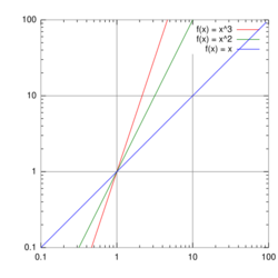
Note the logarithmic scale markings on each of the axes, and that the log x and log y axes (where the logarithms are 0) are where x and y themselves are 1.

In science and engineering, a log–log graph or log–log plot is a two-dimensional graph of numerical data that uses logarithmic scales on both the horizontal and vertical axes. Power functions – relationships of the form [math]\displaystyle{ y=ax^k }[/math] – appear as straight lines in a log–log graph, with the exponent corresponding to the slope, and the coefficient corresponding to the intercept. Thus these graphs are very useful for recognizing these relationships and estimating parameters. Any base can be used for the logarithm, though most commonly base 10 (common logs) are used.

Relation with monomials

Given a monomial equation [math]\displaystyle{ y=ax^k, }[/math] taking the logarithm of the equation (with any base) yields: [math]\displaystyle{ \log y = k \log x + \log a. }[/math] Setting [math]\displaystyle{ X = \log x }[/math] and [math]\displaystyle{ Y = \log y, }[/math] which corresponds to using a log–log graph, yields the equation: [math]\displaystyle{ Y = mX + b }[/math] where m = k is the slope of the line (gradient) and b = log a is the intercept on the (log y)-axis, meaning where log x = 0, so, reversing the logs, a is the y value corresponding to x = 1.

Equations

The equation for a line on a log–log scale would be: [math]\displaystyle{ \log_{10}F(x) = m \log_{10}x + b, }[/math] [math]\displaystyle{ F(x) = x^m\cdot10^b, }[/math] where m is the slope and b is the intercept point on the log plot.

Slope of a log–log plot

Finding the slope of a log–log plot using ratios

To find the slope of the plot, two points are selected on the x-axis, say x₁ and x₂. Using the above equation: [math]\displaystyle{ \log[F (x_1)] = m \log (x_1) + b, }[/math] and [math]\displaystyle{ \log[F (x_2)] = m \log(x_2) + b. }[/math] The slope m is found taking the difference: [math]\displaystyle{ m = \frac { \log (F_2) - \log (F_1)} { \log(x_2) - \log(x_1) } = \frac {\log (F_2/F_1)}{\log(x_2/x_1)}, }[/math] where F₁ is shorthand for F(x₁) and F₂ is shorthand for F(x₂). The figure at right illustrates the formula. Notice that the slope in the example of the figure is negative. The formula also provides a negative slope, as can be seen from the following property of the logarithm: [math]\displaystyle{ \log(x_1/x_2) = -\log(x_2/x_1). }[/math]

Finding the function from the log–log plot

The above procedure now is reversed to find the form of the function F(x) using its (assumed) known log–log plot. To find the function F, pick some fixed point (x₀, F₀), where F₀ is shorthand for F(x₀), somewhere on the straight line in the above graph, and further some other arbitrary point (x₁, F₁) on the same graph. Then from the slope formula above: [math]\displaystyle{ m = \frac {\log (F_1 / F_0)}{\log(x_1 / x_0)} }[/math] which leads to [math]\displaystyle{ \log(F_1 / F_0) = m \log(x_1 / x_0) = \log[(x_1 / x_0)^m ]. }[/math] Notice that 10^{log₁₀(F₁)} = F₁. Therefore, the logs can be inverted to find: [math]\displaystyle{ \frac{F_1}{F_0} = \left(\frac{x_1}{x_0}\right)^m }[/math] or [math]\displaystyle{ F_1 = \frac{F_0}{x_0^m} \, x^m, }[/math] which means that [math]\displaystyle{ F(x) = \mathrm{constant}\cdot x^m. }[/math] In other words, F is proportional to x to the power of the slope of the straight line of its log–log graph. Specifically, a straight line on a log–log plot containing points (x₀, F₀) and (x₁, F₁) will have the function: [math]\displaystyle{ F(x) = {F_0}\left(\frac{x}{x_0} \right)^\frac {\log (F_1/F_0)}{\log(x_1/x_0)}, }[/math] Of course, the inverse is true too: any function of the form [math]\displaystyle{ F(x) = \mathrm{constant} \cdot x^m }[/math] will have a straight line as its log–log graph representation, where the slope of the line is m.

Finding the area under a straight-line segment of log–log plot

To calculate the area under a continuous, straight-line segment of a log–log plot (or estimating an area of an almost-straight line), take the function defined previously [math]\displaystyle{ F(x) = \mathrm{constant}\cdot x^m. }[/math] and integrate it. Since it is only operating on a definite integral (two defined endpoints), the area A under the plot takes the form [math]\displaystyle{ A(x) = \int_{x_0}^{x_1} F(x) \, dx = \left.\frac{\mathrm{constant}}{m+1} \cdot x^{m+1}\right|_{x_0}^{x_1} }[/math]

Rearranging the original equation and plugging in the fixed point values, it is found that [math]\displaystyle{ \mathrm{constant} = \frac{F_0}{x_0^m} }[/math]

Substituting back into the integral, you find that for A over x₀ to x₁

[math]\displaystyle{ \begin{align} A &= \frac{F_0/x_0^m}{m+1}\cdot (x_1^{m+1}-x_0^{m+1}) \\[1.2ex] \log A &= \log \left[\frac{F_0 / x_0^m}{m+1} \cdot (x_1^{m+1}-x_0^{m+1})\right] \\ &= \log \frac{F_0}{m+1} - \log \frac{1}{x_0^m} + \log (x_1^{m+1}-x_0^{m+1}) \\ &= \log \frac{F_0}{m+1} + \log \left(\frac{x_1^{m+1} - x_0^{m+1}}{x_0^m}\right) \\ &= \log \frac{F_0}{m+1} + \log \left(\frac{x_1^m}{x_0^m}\cdot x_1 - \frac{x_0^{m+1}}{x_0^m}\right) \end{align} }[/math]

Therefore, [math]\displaystyle{ A = \frac{F_0}{m+1} \cdot \left[x_1 \cdot \left(\frac {x_1}{x_0}\right)^m - x_0\right] }[/math]

For m = −1, the integral becomes [math]\displaystyle{ \begin{align} A_{(m=-1)} &= \int_{x_0}^{x_1} F(x) \, dx = \int_{x_0}^{x_1} \frac {\mathrm{constant}}{x} \, dx = \frac{F_0}{x_0^{-1}} \int_{x_0}^{x_1} \frac {dx}{x} = F_0 \cdot x_0 \cdot {\ln x }\Big|_{x_0}^{x_1} \\ A_{(m=-1)} &= F_0 \cdot x_0 \cdot \ln \frac{x_1}{x_0} \end{align} }[/math]

Applications

A log-log plot condensing information that spans more than one order of magnitude along both axes

These graphs are useful when the parameters a and b need to be estimated from numerical data. Specifications such as this are used frequently in economics.

One example is the estimation of money demand functions based on inventory theory, in which it can be assumed that money demand at time t is given by [math]\displaystyle{ M_t = AR_t^bY_t^cU_t, }[/math] where M is the real quantity of money held by the public, R is the rate of return on an alternative, higher yielding asset in excess of that on money, Y is the public's real income, U is an error term assumed to be lognormally distributed, A is a scale parameter to be estimated, and b and c are elasticity parameters to be estimated. Taking logs yields [math]\displaystyle{ m_t = a + br_t + cy_t + u_t, }[/math] where m = log M, a = log A, r = log R, y = log Y, and u = log U with u being normally distributed. This equation can be estimated using ordinary least squares.

Another economic example is the estimation of a firm's Cobb–Douglas production function, which is the right side of the equation [math]\displaystyle{ Q_t=AN_t^{\alpha}K_t^{\beta}U_t, }[/math] in which Q is the quantity of output that can be produced per month, N is the number of hours of labor employed in production per month, K is the number of hours of physical capital utilized per month, U is an error term assumed to be lognormally distributed, and A, [math]\displaystyle{ \alpha }[/math], and [math]\displaystyle{ \beta }[/math] are parameters to be estimated. Taking logs gives the linear regression equation [math]\displaystyle{ q_t = a + \alpha n_t + \beta k_t + u_t }[/math] where q = log Q, a = log A, n = log N, k = log K, and u = log U.

Log–log regression can also be used to estimate the fractal dimension of a naturally occurring fractal.

However, going in the other direction – observing that data appears as an approximate line on a log–log scale and concluding that the data follows a power law – is not always valid.

In fact, many other functional forms appear approximately linear on the log–log scale, and simply evaluating the goodness of fit of a linear regression on logged data using the coefficient of determination (R²) may be invalid, as the assumptions of the linear regression model, such as Gaussian error, may not be satisfied; in addition, tests of fit of the log–log form may exhibit low statistical power, as these tests may have low likelihood of rejecting power laws in the presence of other true functional forms. While simple log–log plots may be instructive in detecting possible power laws, and have been used dating back to Pareto in the 1890s, validation as a power laws requires more sophisticated statistics.

These graphs are also extremely useful when data are gathered by varying the control variable along an exponential function, in which case the control variable x is more naturally represented on a log scale, so that the data points are evenly spaced, rather than compressed at the low end. The output variable y can either be represented linearly, yielding a lin–log graph (log x, y), or its logarithm can also be taken, yielding the log–log graph (log x, log y).

Bode plot (a graph of the frequency response of a system) is also log–log plot.

In chemical kinetics, the general form of the dependence of the reaction rate on concentration takes the form of a power law (law of mass action), so a log-log plot is useful for estimating the reaction parameters from experiment.

See also

• Semi-log plot (lin–log or log–lin)
• Power law
• Zipf law

External links

• Non-Newtonian calculus website

de:Logarithmenpapier#Doppeltlogarithmisches Papier

References

- ↑ Bourne, Murray. "7. Log-Log and Semi-log Graphs" (in en-us). https://www.intmath.com/exponential-logarithmic-functions/7-graphs-log-semilog.php.
- ↑ 2.0 2.1 Clauset, A.; Shalizi, C. R.; Newman, M. E. J. (2009). "Power-Law Distributions in Empirical Data". SIAM Review 51 (4): 661–703. doi:10.1137/070710111. Bibcode: 2009SIAMR..51..661C.