Logit-normal distribution

Logit-normal

Probability density function
Cumulative distribution function
Notation	[math]\displaystyle{ P( \mathcal{N}(\mu,\,\sigma^2) ) }[/math]
Parameters	σ2 > 0 — squared scale (real), μ ∈ R — location
Support	x ∈ (0, 1)
PDF	[math]\displaystyle{ \frac{1}{\sigma \sqrt{2 \pi}}\, e^{-\frac{(\operatorname{logit}(x) - \mu)^2}{2\sigma^2}}\frac{1}{x (1-x)} }[/math]
CDF	[math]\displaystyle{ \frac12\Big[1 + \operatorname{erf}\Big( \frac{\operatorname{logit}(x)-\mu}{\sqrt{2\sigma^2}}\Big)\Big] }[/math]
Mean	no analytical solution
Median	[math]\displaystyle{ P(\mu)\, }[/math]
Mode	no analytical solution
Variance	no analytical solution
MGF	no analytical solution

In probability theory, a logit-normal distribution is a probability distribution of a random variable whose logit has a normal distribution. If Y is a random variable with a normal distribution, and t is the standard logistic function, then X = t(Y) has a logit-normal distribution; likewise, if X is logit-normally distributed, then Y = logit(X)= log (X/(1-X)) is normally distributed. It is also known as the logistic normal distribution, which often refers to a multinomial logit version (e.g.).

A variable might be modeled as logit-normal if it is a proportion, which is bounded by zero and one, and where values of zero and one never occur.

Characterization

Probability density function

The probability density function (PDF) of a logit-normal distribution, for 0 < x < 1, is:

[math]\displaystyle{ f_X(x;\mu,\sigma) = \frac{1}{\sigma\sqrt{2 \pi}}\,\frac{1}{x (1-x)}\, e^{-\frac{(\operatorname{logit}(x) - \mu)^2}{2\sigma^2}} }[/math]

where μ and σ are the mean and standard deviation of the variable’s logit (by definition, the variable’s logit is normally distributed).

The density obtained by changing the sign of μ is symmetrical, in that it is equal to f(1-x;-μ,σ), shifting the mode to the other side of 0.5 (the midpoint of the (0,1) interval).

Plot of the Logitnormal PDF for various combinations of μ (facets) and σ (colors)

Moments

The moments of the logit-normal distribution have no analytic solution. The moments can be estimated by numerical integration, however numerical integration can be prohibitive when the values of [math]\displaystyle{ \mu, \sigma^2 }[/math]are such that the density function diverges to infinity at the end points zero and one. An alternative is to use the observation that the logit-normal is a transformation of a normal random variable. This allows us to approximate the [math]\displaystyle{ n }[/math]-th moment via the following quasi Monte Carlo estimate [math]\displaystyle{ E[X^n] \approx \frac{1}{K-1} \sum_{i=1}^{K-1} \left( P\left(\Phi^{-1}_{\mu,\sigma^2}(i/K)\right) \right)^n, }[/math]

where [math]\displaystyle{ P }[/math] is the standard logistic function, and [math]\displaystyle{ \Phi^{-1}_{\mu,\sigma^2} }[/math] is the inverse cumulative distribution function of a normal distribution with mean and variance [math]\displaystyle{ \mu, \sigma^2 }[/math].

Mode or modes

When the derivative of the density equals 0 then the location of the mode x satisfies the following equation:

[math]\displaystyle{ \operatorname{logit}(x) = \sigma^2(2x-1)+\mu . }[/math]

For some values of the parameters there are two solutions, i.e. the distribution is bimodal.

Multivariate generalization

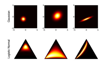
The logistic normal distribution is a generalization of the logit–normal distribution to D-dimensional probability vectors by taking a logistic transformation of a multivariate normal distribution.

Probability density function

The probability density function is:

[math]\displaystyle{ f_X( \mathbf{x}; \boldsymbol{\mu} , \boldsymbol{\Sigma} ) = \frac{1}{ | 2 \pi \boldsymbol{\Sigma} |^\frac{1}{2} } \, \frac{1}{ \prod\limits_{i=1}^D x_i } \, e^{- \frac{1}{2} \left\{ \log \left( \frac{ \mathbf{x}_{-D} }{ x_D } \right) - \boldsymbol{\mu} \right\}^\top \boldsymbol{\Sigma}^{-1} \left\{ \log \left( \frac{ \mathbf{x}_{-D} }{ x_D } \right) - \boldsymbol{\mu} \right\} } \quad , \quad \mathbf{x} \in \mathcal{S}^D \;\; , }[/math]

where [math]\displaystyle{ \mathbf{x}_{-D} }[/math] denotes a vector of the first (D-1) components of [math]\displaystyle{ \mathbf{x} }[/math] and [math]\displaystyle{ \mathcal{S}^D }[/math] denotes the simplex of D-dimensional probability vectors. This follows from applying the additive logistic transformation to map a multivariate normal random variable [math]\displaystyle{ \mathbf{y} \sim \mathcal{N} \left( \boldsymbol{\mu} , \boldsymbol{\Sigma} \right) \; , \; \mathbf{y} \in \mathbb{R}^{D-1} }[/math] to the simplex:

[math]\displaystyle{ \mathbf{x} = \left[ \frac{ e^{ y_1 } }{ 1 + \sum_{i=1}^{D-1} e^{ y_i } } , \dots , \frac{ e^{ y_{D-1} } }{ 1 + \sum_{i=1}^{D-1} e^{ y_i } } , \frac{ 1 }{ 1 + \sum_{i=1}^{D-1} e^{ y_i } } \right]^\top }[/math]

Gaussian density functions and corresponding logistic normal density functions after logistic transformation.

The unique inverse mapping is given by:

[math]\displaystyle{ \mathbf{y} = \left[ \log \left( \frac{ x_1 }{ x_D } \right) , \dots , \log \left( \frac{ x_{D-1} }{ x_D } \right) \right]^\top }[/math].

This is the case of a vector x which components sum up to one. In the case of x with sigmoidal elements, that is, when

[math]\displaystyle{ \mathbf{y} = \left[ \log \left( \frac{ x_1 }{ 1-x_1 } \right) , \dots , \log \left( \frac{ x_D }{ 1-x_D } \right) \right]^\top }[/math]

we have

[math]\displaystyle{ f_X( \mathbf{x}; \boldsymbol{\mu} , \boldsymbol{\Sigma} ) = \frac{1}{ | 2 \pi \boldsymbol{\Sigma} |^\frac{1}{2} } \, \frac{1}{ \prod\limits_{i=1}^D \left(x_i(1-x_i)\right) } \, e^{- \frac{1}{2} \left\{ \log \left( \frac{ \mathbf{x} }{ 1-\mathbf{x} } \right) - \boldsymbol{\mu} \right\}^\top \boldsymbol{\Sigma}^{-1} \left\{ \log \left( \frac{ \mathbf{x}}{ 1-\mathbf{x} } \right) - \boldsymbol{\mu} \right\} } }[/math]

where the log and the division in the argument are taken element-wise. This is because the Jacobian matrix of the transformation is diagonal with elements [math]\displaystyle{ \frac{ 1 }{ x_i(1-x_i)} }[/math].

Use in statistical analysis

The logistic normal distribution is a more flexible alternative to the Dirichlet distribution in that it can capture correlations between components of probability vectors. It also has the potential to simplify statistical analyses of compositional data by allowing one to answer questions about log-ratios of the components of the data vectors. One is often interested in ratios rather than absolute component values.

The probability simplex is a bounded space, making standard techniques that are typically applied to vectors in [math]\displaystyle{ \mathbb{R}^n }[/math] less meaningful. Aitchison described the problem of spurious negative correlations when applying such methods directly to simplicial vectors. However, mapping compositional data in [math]\displaystyle{ \mathcal{S}^D }[/math] through the inverse of the additive logistic transformation yields real-valued data in [math]\displaystyle{ \mathbb{R}^{D-1} }[/math]. Standard techniques can be applied to this representation of the data. This approach justifies use of the logistic normal distribution, which can thus be regarded as the "Gaussian of the simplex".

Relationship with the Dirichlet distribution

Logistic normal approximation to Dirichlet distribution

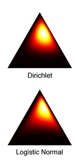
The Dirichlet and logistic normal distributions are never exactly equal for any choice of parameters. However, Aitchison described a method for approximating a Dirichlet with a logistic normal such that their Kullback–Leibler divergence (KL) is minimized:

[math]\displaystyle{ K(p,q) = \int_{\mathcal{S}^D} p \left( \mathbf{x} \mid \boldsymbol{\alpha} \right) \log \left( \frac{ p \left( \mathbf{x} \mid \boldsymbol{\alpha} \right) }{ q \left( \mathbf{x} \mid \boldsymbol{\mu} , \boldsymbol{\Sigma} \right) } \right) \, d \mathbf{x} }[/math]

This is minimized by:

[math]\displaystyle{ \boldsymbol{\mu}^* = \mathbf{E}_p \left[ \log \left( \frac{ \mathbf{x}_{-D} }{ x_D } \right) \right] \quad , \quad \boldsymbol{\Sigma}^* = \textbf{Var}_p \left[ \log \left( \frac{ \mathbf{x}_{-D} }{ x_D } \right) \right] }[/math]

Using moment properties of the Dirichlet distribution, the solution can be written in terms of the digamma [math]\displaystyle{ \psi }[/math] and trigamma [math]\displaystyle{ \psi' }[/math] functions:

[math]\displaystyle{ \mu_i^* = \psi \left( \alpha_i \right) - \psi \left( \alpha_D \right) \quad , \quad i = 1 , \ldots , D-1 }[/math]

[math]\displaystyle{ \Sigma_{ii}^* = \psi' \left( \alpha_i \right) + \psi' \left( \alpha_D \right) \quad , \quad i = 1 , \ldots , D-1 }[/math]

[math]\displaystyle{ \Sigma_{ij}^* = \psi' \left( \alpha_D \right) \quad , \quad i \neq j }[/math]

This approximation is particularly accurate for large [math]\displaystyle{ \boldsymbol{\alpha} }[/math]. In fact, one can show that for [math]\displaystyle{ \alpha_i \rightarrow \infty , i = 1 , \ldots , D }[/math], we have that [math]\displaystyle{ p \left( \mathbf{x} \mid \boldsymbol{\alpha} \right) \rightarrow q \left( \mathbf{x} \mid \boldsymbol{\mu}^* , \boldsymbol{\Sigma}^* \right) }[/math].

See also

• Beta distribution and Kumaraswamy distribution, other two-parameter distributions on a bounded interval with similar shapes

Further reading

• Frederic, P. & Lad, F. (2008) Two Moments of the Logitnormal Distribution. Communications in Statistics-Simulation and Computation. 37: 1263-1269
• Mead, R. (1965). "A Generalised Logit-Normal Distribution". Biometrics 21 (3): 721–732. doi:10.2307/2528553. PMID 5858101. 

External links

• logitnorm package for R

References

- ↑ 1.0 1.1 Aitchison, J.; Shen, S. M. (1980). "Logistic-normal distributions: Some properties and uses". Biometrika 67 (2): 261. doi:10.2307/2335470. ISSN 0006-3444.
- ↑ Huang, Jonathan; Tomasz, Malisiewicz. "Fitting a Hierarchical Logistical Normal Distribution". https://people.csail.mit.edu/tomasz/papers/huang_hln_tech_report_2006.pdf.
- ↑ Peter Hoff, 2003. Link
- ↑ "Log-normal and logistic-normal terminology - AI and Social Science – Brendan O'Connor". http://brenocon.com/blog/2011/05/log-normal-and-logistic-normal-terminology/.
- ↑ 5.0 5.1 J. Atchison. "The Statistical Analysis of Compositional Data." Monographs on Statistics and Applied Probability, Chapman and Hall, 1986. Book
- ↑ Hinde, John (2011). "Logistic Normal Distribution". in Lovric, Miodrag. International Encyclopedia of Statistical Sciences. Springer. pp. 754–755. doi:10.1007/978-3-642-04898-2_342. ISBN 978-3-642-04897-5.