Physics:Bending of plates

Bending of an edge-clamped circular plate under the action of a transverse pressure. The left half of the plate shows the deformed shape, while the right half shows the undeformed shape. This calculation was performed using Ansys.

Bending of plates, or plate bending, refers to the deflection of a plate perpendicular to the plane of the plate under the action of external forces and moments. The amount of deflection can be determined by solving the differential equations of an appropriate plate theory. The stresses in the plate can be calculated from these deflections. Once the stresses are known, failure theories can be used to determine whether a plate will fail under a given load.

Bending of Kirchhoff-Love plates

Forces and moments on a flat plate.

Definitions

For a thin rectangular plate of thickness [math]\displaystyle{ H }[/math], Young's modulus [math]\displaystyle{ E }[/math], and Poisson's ratio [math]\displaystyle{ \nu }[/math], we can define parameters in terms of the plate deflection, [math]\displaystyle{ w }[/math].

The flexural rigidity is given by

[math]\displaystyle{ D = \frac{EH^3}{12\left(1-\nu^2\right)} }[/math]

Moments

The bending moments per unit length are given by

[math]\displaystyle{ M_{x} = -D \left( \frac{\partial^2 w}{\partial x^2} + \nu \frac{\partial^2 w}{\partial y^2} \right) }[/math]

[math]\displaystyle{ M_{y} = -D \left( \nu \frac{\partial^2 w}{\partial x^2} + \frac{\partial^2 w}{\partial y^2} \right) }[/math]

The twisting moment per unit length is given by

[math]\displaystyle{ M_{xy} = -D \left( 1 - \nu \right) \frac{\partial^2 w}{\partial x\partial y} }[/math]

Forces

The shear forces per unit length are given by

[math]\displaystyle{ Q_{x} = -D \frac{\partial}{\partial x} \left( \frac{\partial^2 w}{\partial x^2} + \frac{\partial^2 w}{\partial y^2} \right) }[/math]

[math]\displaystyle{ Q_{y} = -D \frac{\partial}{\partial y} \left( \frac{\partial^2 w}{\partial x^2} + \frac{\partial^2 w}{\partial y^2} \right) }[/math]

Stresses

The bending stresses are given by

[math]\displaystyle{ \sigma_{x} = -\frac{12Dz}{H^3} \left( \frac{\partial^2 w}{\partial x^2} + \nu \frac{\partial^2 w}{\partial y^2} \right) }[/math]

[math]\displaystyle{ \sigma_{y} = -\frac{12Dz}{H^3} \left( \nu \frac{\partial^2 w}{\partial x^2} + \frac{\partial^2 w}{\partial y^2} \right) }[/math]

The shear stress is given by

[math]\displaystyle{ \tau_{xy} = -\frac{12Dz}{H^3} \left(1-\nu\right) \frac{\partial^2 w}{\partial x\partial y} }[/math]

Strains

The bending strains for small-deflection theory are given by

[math]\displaystyle{ \epsilon_{x} = \frac{\partial u}{\partial x} = -z\frac{\partial^2 w}{\partial x^2} }[/math]

[math]\displaystyle{ \epsilon_{y} = \frac{\partial v}{\partial y} = -z\frac{\partial^2 w}{\partial y^2} }[/math]

The shear strain for small-deflection theory is given by

[math]\displaystyle{ \gamma_{xy} = \frac{\partial u}{\partial y} + \frac{\partial v}{\partial x} = -2z\frac{\partial^2 w}{\partial x\partial y} }[/math]

For large-deflection plate theory, we consider the inclusion of membrane strains

[math]\displaystyle{ \epsilon_{x} = \frac{\partial u}{\partial x} + \frac{1}{2}\left(\frac{\partial w}{\partial x}\right)^2 }[/math]

[math]\displaystyle{ \epsilon_{y} = \frac{\partial v}{\partial y} + \frac{1}{2}\left(\frac{\partial w}{\partial y}\right)^2 }[/math]

[math]\displaystyle{ \gamma_{xy} = \frac{\partial u}{\partial y} + \frac{\partial v}{\partial x} + \frac{\partial w}{\partial x} \frac{\partial w}{\partial y} }[/math]

Deflections

The deflections are given by

[math]\displaystyle{ u = -z\frac{\partial w}{\partial x} }[/math]

[math]\displaystyle{ v = -z\frac{\partial w}{\partial y} }[/math]

Derivation

In the Kirchhoff–Love plate theory for plates the governing equations are

[math]\displaystyle{ N_{\alpha\beta,\alpha} = 0 }[/math]

and

[math]\displaystyle{ M_{\alpha\beta,\alpha\beta} - q = 0 }[/math]

In expanded form,

[math]\displaystyle{ \cfrac{\partial N_{11}}{\partial x_1} + \cfrac{\partial N_{21}}{\partial x_2} = 0 ~;~~ \cfrac{\partial N_{12}}{\partial x_1} + \cfrac{\partial N_{22}}{\partial x_2} = 0 }[/math]

and

[math]\displaystyle{ \cfrac{\partial^2 M_{11}}{\partial x_1^2} + 2\cfrac{\partial^2 M_{12}}{\partial x_1 \partial x_2} + \cfrac{\partial^2 M_{22}}{\partial x_2^2} = q }[/math]

where [math]\displaystyle{ q(x) }[/math] is an applied transverse load per unit area, the thickness of the plate is [math]\displaystyle{ H=2h }[/math], the stresses are [math]\displaystyle{ \sigma_{ij} }[/math], and

[math]\displaystyle{ N_{\alpha\beta} := \int_{-h}^h \sigma_{\alpha\beta}~dx_3 ~;~~ M_{\alpha\beta} := \int_{-h}^h x_3~\sigma_{\alpha\beta}~dx_3~. }[/math]

The quantity [math]\displaystyle{ N }[/math] has units of force per unit length. The quantity [math]\displaystyle{ M }[/math] has units of moment per unit length.

For isotropic, homogeneous, plates with Young's modulus [math]\displaystyle{ E }[/math] and Poisson's ratio [math]\displaystyle{ \nu }[/math] these equations reduce to

[math]\displaystyle{ \nabla^2\nabla^2 w = -\cfrac{q}{D} ~;~~ D := \cfrac{2h^3E}{3(1-\nu^2)} = \cfrac{H^3E}{12(1-\nu^2)} }[/math]

where [math]\displaystyle{ w(x_1,x_2) }[/math] is the deflection of the mid-surface of the plate.

Small deflection of thin rectangular plates

This is governed by the Germain-Lagrange plate equation

[math]\displaystyle{ \cfrac{\partial^4 w}{\partial x^4} + 2\cfrac{\partial^4 w}{\partial x^2\partial y^2} + \cfrac{\partial^4 w}{\partial y^4} = \cfrac{q}{D} }[/math]

This equation was first derived by Lagrange in December 1811 in correcting the work of Germain who provided the basis of the theory.

Large deflection of thin rectangular plates

This is governed by the Föppl–von Kármán plate equations

[math]\displaystyle{ \cfrac{\partial^4 F}{\partial x^4} + 2\cfrac{\partial^4 F}{\partial x^2\partial y^2} + \cfrac{\partial^4 F}{\partial y^4} = E\left[\left(\cfrac{\partial^2 w}{\partial x \partial y}\right)^2 - \cfrac{\partial^2 w}{\partial x^2} \cfrac{\partial^2 w}{\partial y^2}\right] }[/math]

[math]\displaystyle{ \cfrac{\partial^4 w}{\partial x^4} + 2\cfrac{\partial^4 w}{\partial x^2\partial y^2} + \cfrac{\partial^4 w}{\partial y^4} = \cfrac{q}{D} + \cfrac{H}{D}\left( \cfrac{\partial^2 F}{\partial y^2}\cfrac{\partial^2 w}{\partial x^2} + \cfrac{\partial^2 F}{\partial x^2}\cfrac{\partial^2 w}{\partial y^2} - 2\cfrac{\partial^2 F}{\partial x \partial y}\cfrac{\partial^2 w}{\partial x \partial y} \right) }[/math]

where [math]\displaystyle{ F }[/math] is the stress function.

Circular Kirchhoff-Love plates

The bending of circular plates can be examined by solving the governing equation with appropriate boundary conditions. These solutions were first found by Poisson in 1829. Cylindrical coordinates are convenient for such problems. Here [math]\displaystyle{ z }[/math] is the distance of a point from the midplane of the plate.

The governing equation in coordinate-free form is

[math]\displaystyle{ \nabla^2 \nabla^2 w = -\frac{q}{D} \,. }[/math]

In cylindrical coordinates [math]\displaystyle{ (r, \theta, z) }[/math],

[math]\displaystyle{ \nabla^2 w \equiv \frac{1}{r}\frac{\partial }{\partial r}\left(r \frac{\partial w}{\partial r}\right) + \frac{1}{r^2}\frac{\partial^2 w}{\partial \theta^2} + \frac{\partial^2 w}{\partial z^2} \,. }[/math]

For symmetrically loaded circular plates, [math]\displaystyle{ w = w(r) }[/math], and we have

[math]\displaystyle{ \nabla^2 w \equiv \frac{1}{r}\cfrac{d }{d r}\left(r \cfrac{d w}{d r}\right) \,. }[/math]

Therefore, the governing equation is

[math]\displaystyle{ \frac{1}{r}\cfrac{d }{d r}\left[r \cfrac{d }{d r}\left\{\frac{1}{r}\cfrac{d }{d r}\left(r \cfrac{d w}{d r}\right)\right\}\right] = -\frac{q}{D}\,. }[/math]

If [math]\displaystyle{ q }[/math] and [math]\displaystyle{ D }[/math] are constant, direct integration of the governing equation gives us

[math]\displaystyle{ w(r) = -\frac{qr^4}{64 D} + C_1\ln r + \cfrac{C_2 r^2}{2} + \cfrac{C_3r^2}{4}(2\ln r - 1) + C_4 }[/math]

where [math]\displaystyle{ C_i }[/math] are constants. The slope of the deflection surface is

[math]\displaystyle{ \phi(r) = \cfrac{d w}{d r} = -\frac{qr^3}{16D} + \frac{C_1}{r} + C_2 r + C_3 r \ln r \,. }[/math]

For a circular plate, the requirement that the deflection and the slope of the deflection are finite at [math]\displaystyle{ r = 0 }[/math] implies that [math]\displaystyle{ C_1 = 0 }[/math]. However, [math]\displaystyle{ C_3 }[/math] need not equal 0, as the limit of [math]\displaystyle{ r \ln r\, }[/math] exists as you approach [math]\displaystyle{ r = 0 }[/math] from the right.

Clamped edges

For a circular plate with clamped edges, we have [math]\displaystyle{ w(a) = 0 }[/math] and [math]\displaystyle{ \phi(a) = 0 }[/math] at the edge of the plate (radius [math]\displaystyle{ a }[/math]). Using these boundary conditions we get

[math]\displaystyle{ w(r) = -\frac{q}{64 D} (a^2 -r^2)^2 \quad \text{and} \quad \phi(r) = \frac{qr}{16 D}(a^2-r^2) \,. }[/math]

The in-plane displacements in the plate are

[math]\displaystyle{ u_r(r) = -z\phi(r) \quad \text{and} \quad u_\theta(r) = 0 \,. }[/math]

The in-plane strains in the plate are

[math]\displaystyle{ \varepsilon_{rr} = \cfrac{d u_r}{d r} = -\frac{qz}{16D}(a^2-3r^2) ~,~~ \varepsilon_{\theta\theta} = \frac{u_r}{r} = -\frac{qz}{16D}(a^2-r^2) ~,~~ \varepsilon_{r\theta} = 0 \,. }[/math]

The in-plane stresses in the plate are

[math]\displaystyle{ \sigma_{rr} = \frac{E}{1-\nu^2}\left[\varepsilon_{rr} + \nu\varepsilon_{\theta\theta}\right] ~;~~ \sigma_{\theta\theta} = \frac{E}{1-\nu^2}\left[\varepsilon_{\theta\theta} + \nu\varepsilon_{rr}\right] ~;~~ \sigma_{r\theta} = 0 \,. }[/math]

For a plate of thickness [math]\displaystyle{ 2h }[/math], the bending stiffness is [math]\displaystyle{ D = 2Eh^3/[3(1-\nu^2)] }[/math] and we have

[math]\displaystyle{ \begin{align} \sigma_{rr} &= -\frac{3qz}{32h^3}\left[(1+\nu)a^2-(3+\nu)r^2\right] \\ \sigma_{\theta\theta} &= -\frac{3qz}{32h^3}\left[(1+\nu)a^2-(1+3\nu)r^2\right]\\ \sigma_{r\theta} &= 0 \,. \end{align} }[/math]

The moment resultants (bending moments) are

[math]\displaystyle{ M_{rr} = -\frac{q}{16}\left[(1+\nu)a^2-(3+\nu)r^2\right] ~;~~ M_{\theta\theta} = -\frac{q}{16}\left[(1+\nu)a^2-(1+3\nu)r^2\right] ~;~~ M_{r\theta} = 0 \,. }[/math]

The maximum radial stress is at [math]\displaystyle{ z = h }[/math] and [math]\displaystyle{ r = a }[/math]:

[math]\displaystyle{ \left.\sigma_{rr}\right|_{z=h,r=a} = \frac{3qa^2}{16h^2} = \frac{3qa^2}{4H^2} }[/math]

where [math]\displaystyle{ H := 2h }[/math]. The bending moments at the boundary and the center of the plate are

[math]\displaystyle{ \left.M_{rr}\right|_{r=a} = \frac{qa^2}{8} ~,~~ \left.M_{\theta\theta}\right|_{r=a} = \frac{\nu qa^2}{8} ~,~~ \left.M_{rr}\right|_{r=0} = \left.M_{\theta\theta}\right|_{r=0} = -\frac{(1+\nu) qa^2}{16} \,. }[/math]

Rectangular Kirchhoff-Love plates

Bending of a rectangular plate under the action of a distributed force [math]\displaystyle{ q }[/math] per unit area.

For rectangular plates, Navier in 1820 introduced a simple method for finding the displacement and stress when a plate is simply supported. The idea was to express the applied load in terms of Fourier components, find the solution for a sinusoidal load (a single Fourier component), and then superimpose the Fourier components to get the solution for an arbitrary load.

Sinusoidal load

Let us assume that the load is of the form

[math]\displaystyle{ q(x,y) = q_0 \sin\frac{\pi x}{a}\sin\frac{\pi y}{b} \,. }[/math]

Here [math]\displaystyle{ q_0 }[/math] is the amplitude, [math]\displaystyle{ a }[/math] is the width of the plate in the [math]\displaystyle{ x }[/math]-direction, and [math]\displaystyle{ b }[/math] is the width of the plate in the [math]\displaystyle{ y }[/math]-direction.

Since the plate is simply supported, the displacement [math]\displaystyle{ w(x,y) }[/math] along the edges of the plate is zero, the bending moment [math]\displaystyle{ M_{xx} }[/math] is zero at [math]\displaystyle{ x=0 }[/math] and [math]\displaystyle{ x=a }[/math], and [math]\displaystyle{ M_{yy} }[/math] is zero at [math]\displaystyle{ y=0 }[/math] and [math]\displaystyle{ y=b }[/math].

If we apply these boundary conditions and solve the plate equation, we get the solution

[math]\displaystyle{ w(x,y) = \frac{q_0}{\pi^4 D}\,\left(\frac{1}{a^2}+\frac{1}{b^2}\right)^{-2}\,\sin\frac{\pi x}{a}\sin\frac{\pi y}{b} \,. }[/math]

Where D is the flexural rigidity

[math]\displaystyle{ D=\frac{Et^3}{12(1-\nu^2)} }[/math]

Analogous to flexural stiffness EI. We can calculate the stresses and strains in the plate once we know the displacement.

For a more general load of the form

[math]\displaystyle{ q(x,y) = q_0 \sin\frac{m \pi x}{a}\sin\frac{n \pi y}{b} }[/math]

where [math]\displaystyle{ m }[/math] and [math]\displaystyle{ n }[/math] are integers, we get the solution

[math]\displaystyle{ \text{(1)} \qquad w(x,y) = \frac{q_0}{\pi^4 D}\,\left(\frac{m^2}{a^2}+\frac{n^2}{b^2}\right)^{-2}\,\sin\frac{m \pi x}{a}\sin\frac{n \pi y}{b} \,. }[/math]

Navier solution

Double trigonometric series equation

We define a general load [math]\displaystyle{ q(x,y) }[/math] of the following form

[math]\displaystyle{ q(x,y) = \sum_{m=1}^{\infty} \sum_{n=1}^\infty a_{mn}\sin\frac{m \pi x}{a}\sin\frac{n \pi y}{b} }[/math]

where [math]\displaystyle{ a_{mn} }[/math] is a Fourier coefficient given by

[math]\displaystyle{ a_{mn} = \frac{4}{ab}\int_0^b \int_0^a q(x,y)\sin\frac{m\pi x}{a}\sin\frac{n\pi y}{b}\,\text{d}x\text{d}y }[/math].

The classical rectangular plate equation for small deflections thus becomes:

[math]\displaystyle{ \cfrac{\partial^4 w}{\partial x^4} + 2\cfrac{\partial^4 w}{\partial x^2\partial y^2} + \cfrac{\partial^4 w}{\partial y^4} = \cfrac{1}{D} \sum_{m=1}^{\infty} \sum_{n=1}^\infty a_{mn}\sin\frac{m \pi x}{a}\sin\frac{n \pi y}{b} }[/math]

Simply-supported plate with general load

We assume a solution [math]\displaystyle{ w(x,y) }[/math] of the following form

[math]\displaystyle{ w(x,y) = \sum_{m=1}^{\infty} \sum_{n=1}^\infty w_{mn}\sin\frac{m \pi x}{a}\sin\frac{n \pi y}{b} }[/math]

The partial differentials of this function are given by

[math]\displaystyle{ \cfrac{\partial^4 w}{\partial x^4} = \sum_{m=1}^{\infty} \sum_{n=1}^\infty \left(\frac{m \pi}{a}\right)^4 w_{mn}\sin\frac{m \pi x}{a}\sin\frac{n \pi y}{b} }[/math]

[math]\displaystyle{ \cfrac{\partial^4 w}{\partial x^2 \partial y^2} = \sum_{m=1}^{\infty} \sum_{n=1}^\infty \left(\frac{m \pi}{a}\right)^2 \left(\frac{n \pi}{b}\right)^2 w_{mn}\sin\frac{m \pi x}{a}\sin\frac{n \pi y}{b} }[/math]

[math]\displaystyle{ \cfrac{\partial^4 w}{\partial y^4} = \sum_{m=1}^{\infty} \sum_{n=1}^\infty \left(\frac{n \pi}{b}\right)^4 w_{mn}\sin\frac{m \pi x}{a}\sin\frac{n \pi y}{b} }[/math]

Substituting these expressions in the plate equation, we have

[math]\displaystyle{ \sum_{m=1}^{\infty} \sum_{n=1}^\infty \left( \left(\frac{m \pi}{a}\right)^2 + \left(\frac{n \pi}{b}\right)^2 \right)^2 w_{mn}\sin\frac{m \pi x}{a}\sin\frac{n \pi y}{b} = \sum_{m=1}^{\infty} \sum_{n=1}^\infty \cfrac{a_{mn}}{D} \sin\frac{m \pi x}{a}\sin\frac{n \pi y}{b} }[/math]

Equating the two expressions, we have

[math]\displaystyle{ \left( \left(\frac{m \pi}{a}\right)^2 + \left(\frac{n \pi}{b}\right)^2 \right)^2 w_{mn} = \cfrac{a_{mn}}{D} }[/math]

which can be rearranged to give

[math]\displaystyle{ w_{mn} = \frac{1}{\pi^4 D}\frac{a_{mn}}{\left(\frac{m^2}{a^2} + \frac{n^2}{b^2}\right)^2} }[/math]

The deflection of a simply-supported plate (of corner-origin) with general load is given by

[math]\displaystyle{ w(x,y) = \frac{1}{\pi^4 D} \sum_{m=1}^\infty \sum_{n=1}^\infty \frac{a_{mn}}{\left(\frac{m^2}{a^2} + \frac{n^2}{b^2}\right)^2} \sin\frac{m \pi x}{a}\sin\frac{n \pi y}{b} }[/math]

Simply-supported plate with uniformly-distributed load

Displacement ([math]\displaystyle{ w }[/math])

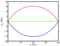Stress ([math]\displaystyle{ \sigma_{xx} }[/math])

Stress ([math]\displaystyle{ \sigma_{yy} }[/math])

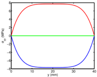Displacement and stresses along [math]\displaystyle{ x=a/2 }[/math] for a rectangular plate with [math]\displaystyle{ a=20 }[/math] mm, [math]\displaystyle{ b=40 }[/math] mm, [math]\displaystyle{ H=2h=0.4 }[/math] mm, [math]\displaystyle{ E=70 }[/math] GPa, and [math]\displaystyle{ \nu=0.35 }[/math] under a load [math]\displaystyle{ q_0 = -10 }[/math] kPa. The red line represents the bottom of the plate, the green line the middle, and the blue line the top of the plate.

For a uniformly-distributed load, we have

[math]\displaystyle{ q(x,y) = q_0 }[/math]

The corresponding Fourier coefficient is thus given by

[math]\displaystyle{ a_{mn} = \frac{4}{ab} \int_0^a \int_0^b q_0\sin\frac{m\pi x}{a}\sin\frac{n\pi y}{b}\,\text{d}x\text{d}y }[/math].

Evaluating the double integral, we have

[math]\displaystyle{ a_{mn} = \frac{4q_0}{\pi^2 mn}(1 - \cos m\pi)(1 - \cos n\pi) }[/math],

or alternatively in a piecewise format, we have

[math]\displaystyle{ a_{mn} = \begin{cases} \cfrac{16q_0}{\pi^2 mn} & m~\text{and}~n~\text{odd} \\ 0 & m~\text{or}~n~\text{even} \end{cases} }[/math]

The deflection of a simply-supported plate (of corner-origin) with uniformly-distributed load is given by

[math]\displaystyle{ w(x,y) = \frac{16 q_0}{\pi^6 D} \sum_{m=1,3,5,...}^\infty \sum_{n=1,3,5,...}^\infty \frac{1}{mn\left(\frac{m^2}{a^2} + \frac{n^2}{b^2}\right)^2} \sin\frac{m \pi x}{a}\sin\frac{n \pi y}{b} }[/math]

The bending moments per unit length in the plate are given by

[math]\displaystyle{ M_{x} = \frac{16 q_0}{\pi^4} \sum_{m=1,3,5,...}^\infty \sum_{n=1,3,5,...}^\infty \frac{\frac{m^2}{a^2} + \nu\frac{n^2}{b^2}} {mn\left(\frac{m^2}{a^2} + \frac{n^2}{b^2}\right)^2} \sin\frac{m \pi x}{a}\sin\frac{n \pi y}{b} }[/math]

[math]\displaystyle{ M_{y} = \frac{16 q_0}{\pi^4} \sum_{m=1,3,5,...}^\infty \sum_{n=1,3,5,...}^\infty \frac{\frac{n^2}{b^2} + \nu\frac{m^2}{a^2}} {mn\left(\frac{m^2}{a^2} + \frac{n^2}{b^2}\right)^2} \sin\frac{m \pi x}{a}\sin\frac{n \pi y}{b} }[/math]

Lévy solution

Another approach was proposed by Lévy in 1899. In this case we start with an assumed form of the displacement and try to fit the parameters so that the governing equation and the boundary conditions are satisfied. The goal is to find [math]\displaystyle{ Y_m(y) }[/math] such that it satisfies the boundary conditions at [math]\displaystyle{ y = 0 }[/math] and [math]\displaystyle{ y = b }[/math] and, of course, the governing equation [math]\displaystyle{ \nabla^2 \nabla^2 w = q/D }[/math].

Let us assume that

[math]\displaystyle{ w(x,y) = \sum_{m=1}^\infty Y_m(y) \sin \frac{m\pi x}{a} \,. }[/math]

For a plate that is simply-supported along [math]\displaystyle{ x=0 }[/math] and [math]\displaystyle{ x=a }[/math], the boundary conditions are [math]\displaystyle{ w=0 }[/math] and [math]\displaystyle{ M_{xx}=0 }[/math]. Note that there is no variation in displacement along these edges meaning that [math]\displaystyle{ \partial w/\partial y = 0 }[/math] and [math]\displaystyle{ \partial^2 w/\partial y^2 = 0 }[/math], thus reducing the moment boundary condition to an equivalent expression [math]\displaystyle{ \partial^2 w/\partial x^2 = 0 }[/math].

Moments along edges

Consider the case of pure moment loading. In that case [math]\displaystyle{ q = 0 }[/math] and [math]\displaystyle{ w(x,y) }[/math] has to satisfy [math]\displaystyle{ \nabla^2 \nabla^2 w = 0 }[/math]. Since we are working in rectangular Cartesian coordinates, the governing equation can be expanded as

[math]\displaystyle{ \frac{\partial^4 w}{\partial x^4} + 2 \frac{\partial^4 w}{\partial x^2\partial y^2} + \frac{\partial^4 w}{\partial y^4} = 0 \,. }[/math]

Plugging the expression for [math]\displaystyle{ w(x,y) }[/math] in the governing equation gives us

[math]\displaystyle{ \sum_{m=1}^\infty \left[\left(\frac{m\pi}{a}\right)^4 Y_m \sin\frac{m\pi x}{a} - 2\left(\frac{m\pi}{a}\right)^2 \cfrac{d^2 Y_m}{d y^2} \sin\frac{m\pi x}{a} + \frac{d^4Y_m}{dy^4} \sin\frac{m\pi x}{a}\right] = 0 }[/math]

or

[math]\displaystyle{ \frac{d^4Y_m}{dy^4} - 2 \frac{m^2\pi^2}{a^2} \cfrac{d^2Y_m}{dy^2} + \frac{m^4\pi^4}{a^4} Y_m = 0 \,. }[/math]

This is an ordinary differential equation which has the general solution

[math]\displaystyle{ Y_m = A_m \cosh\frac{m\pi y}{a} + B_m\frac{m\pi y}{a} \cosh\frac{m\pi y}{a} + C_m \sinh\frac{m\pi y}{a} + D_m\frac{m\pi y}{a} \sinh\frac{m\pi y}{a} }[/math]

where [math]\displaystyle{ A_m, B_m, C_m, D_m }[/math] are constants that can be determined from the boundary conditions. Therefore, the displacement solution has the form

[math]\displaystyle{ w(x,y) = \sum_{m=1}^\infty \left[ \left(A_m + B_m\frac{m\pi y}{a}\right) \cosh\frac{m\pi y}{a} + \left(C_m + D_m\frac{m\pi y}{a}\right) \sinh\frac{m\pi y}{a} \right] \sin \frac{m\pi x}{a} \,. }[/math]

Let us choose the coordinate system such that the boundaries of the plate are at [math]\displaystyle{ x = 0 }[/math] and [math]\displaystyle{ x = a }[/math] (same as before) and at [math]\displaystyle{ y = \pm b/2 }[/math] (and not [math]\displaystyle{ y=0 }[/math] and [math]\displaystyle{ y=b }[/math]). Then the moment boundary conditions at the [math]\displaystyle{ y = \pm b/2 }[/math] boundaries are

[math]\displaystyle{ w = 0 \,, -D\frac{\partial^2 w}{\partial y^2}\Bigr|_{y=b/2} = f_1(x) \,, -D\frac{\partial^2 w}{\partial y^2}\Bigr|_{y=-b/2} = f_2(x) }[/math]

where [math]\displaystyle{ f_1(x), f_2(x) }[/math] are known functions. The solution can be found by applying these boundary conditions. We can show that for the symmetrical case where

[math]\displaystyle{ M_{yy}\Bigr|_{y=-b/2} = M_{yy}\Bigr|_{y=b/2} }[/math]

and

[math]\displaystyle{ f_1(x) = f_2(x) = \sum_{m=1}^\infty E_m\sin\frac{m\pi x}{a} }[/math]

we have

[math]\displaystyle{ w(x,y) = \frac{a^2}{2\pi^2 D}\sum_{m=1}^\infty \frac{E_m}{m^2\cosh\alpha_m}\, \sin\frac{m\pi x}{a}\, \left(\alpha_m \tanh\alpha_m \cosh\frac{m\pi y}{a} - \frac{m\pi y}{a}\sinh\frac{m\pi y}{a}\right) }[/math]

where

[math]\displaystyle{ \alpha_m = \frac{m\pi b}{2a} \,. }[/math]

Similarly, for the antisymmetrical case where

[math]\displaystyle{ M_{yy}\Bigr|_{y=-b/2} = -M_{yy}\Bigr|_{y=b/2} }[/math]

we have

[math]\displaystyle{ w(x,y) = \frac{a^2}{2\pi^2 D}\sum_{m=1}^\infty \frac{E_m}{m^2\sinh\alpha_m}\, \sin\frac{m\pi x}{a}\, \left(\alpha_m \coth\alpha_m \sinh\frac{m\pi y}{a} - \frac{m\pi y}{a}\cosh\frac{m\pi y}{a}\right) \,. }[/math]

We can superpose the symmetric and antisymmetric solutions to get more general solutions.

Simply-supported plate with uniformly-distributed load

For a uniformly-distributed load, we have

[math]\displaystyle{ q(x,y) = q_0 }[/math]

The deflection of a simply-supported plate with centre [math]\displaystyle{ \left(\frac{a}{2}, 0\right) }[/math] with uniformly-distributed load is given by

[math]\displaystyle{ \begin{align} &w(x,y) = \frac{q_0 a^4}{D} \sum_{m=1,3,5,...}^\infty \left( A_m\cosh\frac{m\pi y}{a} + B_m\frac{m\pi y}{a}\sinh\frac{m\pi y}{a} + G_m\right) \sin\frac{m\pi x}{a}\\\\ &\begin{align} \text{where}\quad &A_m = -\frac{2\left(\alpha _m\tanh\alpha _m + 2\right)}{\pi^5 m^5 \cosh\alpha _m}\\ &B_m = \frac{2}{\pi^5 m^5 \cosh\alpha _m}\\ &G_m = \frac{4}{\pi^5 m^5}\\\\ \text{and}\quad &\alpha _m = \frac{m\pi b}{2a} \end{align} \end{align} }[/math]

The bending moments per unit length in the plate are given by

[math]\displaystyle{ M_x = -q_0\pi^2 a^2\sum_{m=1,3,5,...}^\infty m^2\left( \left(\left(\nu -1\right)A_m + 2\nu B_m\right)\cosh\frac{m\pi y}{a} + \left(\nu -1\right)B_m\frac{m\pi y}{a}\sinh\frac{m\pi y}{a} - G_m\right) \sin\frac{m\pi x}{a} }[/math]

[math]\displaystyle{ M_y = -q_0\pi^2 a^2\sum_{m=1,3,5,...}^\infty m^2\left( \left(\left(1-\nu\right)A_m + 2B_m\right)\cosh\frac{m\pi y}{a} + \left(1-\nu\right)B_m\frac{m\pi y}{a}\sinh\frac{m\pi y}{a} - \nu G_m\right) \sin\frac{m\pi x}{a} }[/math]

Uniform and symmetric moment load

For the special case where the loading is symmetric and the moment is uniform, we have at [math]\displaystyle{ y=\pm b/2 }[/math],

[math]\displaystyle{ M_{yy} = f_1(x) = \frac{4M_0}{\pi}\sum_{m=1}^\infty \frac{1}{2m-1}\,\sin\frac{(2m-1)\pi x}{a} \,. }[/math]

Displacement ([math]\displaystyle{ w }[/math])

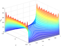Bending stress ([math]\displaystyle{ \sigma_{yy} }[/math])

Transverse shear stress ([math]\displaystyle{ \sigma_{yz} }[/math])

Displacement and stresses for a rectangular plate under uniform bending moment along the edges [math]\displaystyle{ y=-b/2 }[/math] and [math]\displaystyle{ y=b/2 }[/math]. The bending stress [math]\displaystyle{ \sigma_{yy} }[/math] is along the bottom surface of the plate. The transverse shear stress [math]\displaystyle{ \sigma_{yz} }[/math] is along the mid-surface of the plate.

The resulting displacement is

[math]\displaystyle{ \begin{align} & w(x,y) = \frac{2M_0 a^2}{\pi^3 D}\sum_{m=1}^\infty \frac{1}{(2m-1)^3\cosh\alpha_m}\sin\frac{(2m-1)\pi x}{a} \times\\ & ~~ \left[ \alpha_m\,\tanh\alpha_m\cosh\frac{(2m-1)\pi y}{a} -\frac{(2m-1)\pi y}{a} \sinh\frac{(2m-1)\pi y}{a}\right] \end{align} }[/math]

where

[math]\displaystyle{ \alpha_m = \frac{\pi (2m-1)b}{2a} \,. }[/math]

The bending moments and shear forces corresponding to the displacement [math]\displaystyle{ w }[/math] are

[math]\displaystyle{ \begin{align} M_{xx} & = -D\left(\frac{\partial^2 w}{\partial x^2}+\nu\,\frac{\partial^2 w}{\partial y^2}\right) \\ & = \frac{2M_0(1-\nu)}{\pi}\sum_{m=1}^\infty\frac{1}{(2m-1)\cosh\alpha_m}\,\times \\ & ~ \sin\frac{(2m-1)\pi x}{a} \,\times \\ & ~ \left[ -\frac{(2m-1)\pi y}{a}\sinh\frac{(2m-1)\pi y}{a} + \right. \\ & \qquad \qquad \qquad \qquad \left. \left\{\frac{2\nu}{1-\nu} + \alpha_m\tanh\alpha_m\right\}\cosh\frac{(2m-1)\pi y}{a} \right] \\ M_{xy} & = (1-\nu)D\frac{\partial^2 w}{\partial x \partial y} \\ & = -\frac{2M_0(1-\nu)}{\pi}\sum_{m=1}^\infty\frac{1}{(2m-1) \cosh\alpha_m}\,\times \\ & ~ \cos\frac{(2m-1)\pi x}{a} \, \times \\ & ~ \left[\frac{(2m-1)\pi y}{a}\cosh\frac{(2m-1)\pi y}{a} + \right. \\ & \qquad \qquad \qquad \qquad \left. (1-\alpha_m\tanh\alpha_m)\sinh\frac{(2m-1)\pi y}{a}\right] \\ Q_{zx} & = \frac{\partial M_{xx}}{\partial x}-\frac{\partial M_{xy}}{\partial y} \\ & = \frac{4M_0}{a}\sum_{m=1}^\infty \frac{1}{\cosh\alpha_m}\,\times \\ & ~ \cos\frac{(2m-1)\pi x}{a}\cosh\frac{(2m-1)\pi y}{a}\,. \end{align} }[/math]

The stresses are

[math]\displaystyle{ \sigma_{xx} = \frac{12z}{h^3}\,M_{xx} \quad \text{and} \quad \sigma_{zx} = \frac{1}{\kappa h}\,Q_{zx}\left(1 - \frac{4z^2}{h^2}\right)\,. }[/math]

Cylindrical plate bending

Cylindrical bending occurs when a rectangular plate that has dimensions [math]\displaystyle{ a \times b \times h }[/math], where [math]\displaystyle{ a \ll b }[/math] and the thickness [math]\displaystyle{ h }[/math] is small, is subjected to a uniform distributed load perpendicular to the plane of the plate. Such a plate takes the shape of the surface of a cylinder.

Simply supported plate with axially fixed ends

For a simply supported plate under cylindrical bending with edges that are free to rotate but have a fixed [math]\displaystyle{ x_1 }[/math]. Cylindrical bending solutions can be found using the Navier and Levy techniques.

Bending of thick Mindlin plates

For thick plates, we have to consider the effect of through-the-thickness shears on the orientation of the normal to the mid-surface after deformation. Raymond D. Mindlin's theory provides one approach for find the deformation and stresses in such plates. Solutions to Mindlin's theory can be derived from the equivalent Kirchhoff-Love solutions using canonical relations.

Governing equations

The canonical governing equation for isotropic thick plates can be expressed as

[math]\displaystyle{ \begin{align} & \nabla^2 \left(\mathcal{M} - \frac{\mathcal{B}}{1+\nu}\,q\right) = -q \\ & \kappa G h\left(\nabla^2 w + \frac{\mathcal{M}}{D}\right) = -\left(1 - \cfrac{\mathcal{B} c^2}{1+\nu}\right)q \\ & \nabla^2 \left(\frac{\partial \varphi_1}{\partial x_2} - \frac{\partial \varphi_2}{\partial x_1}\right) = c^2\left(\frac{\partial \varphi_1}{\partial x_2} - \frac{\partial \varphi_2}{\partial x_1}\right) \end{align} }[/math]

where [math]\displaystyle{ q }[/math] is the applied transverse load, [math]\displaystyle{ G }[/math] is the shear modulus, [math]\displaystyle{ D = Eh^3/[12(1-\nu^2)] }[/math] is the bending rigidity, [math]\displaystyle{ h }[/math] is the plate thickness, [math]\displaystyle{ c^2 = 2\kappa G h/[D(1-\nu)] }[/math], [math]\displaystyle{ \kappa }[/math] is the shear correction factor, [math]\displaystyle{ E }[/math] is the Young's modulus, [math]\displaystyle{ \nu }[/math] is the Poisson's ratio, and

[math]\displaystyle{ \mathcal{M} = D\left[\mathcal{A}\left(\frac{\partial \varphi_1}{\partial x_1} + \frac{\partial \varphi_2}{\partial x_2}\right) - (1-\mathcal{A})\nabla^2 w\right] + \frac{2q}{1-\nu^2}\mathcal{B} \,. }[/math]

In Mindlin's theory, [math]\displaystyle{ w }[/math] is the transverse displacement of the mid-surface of the plate and the quantities [math]\displaystyle{ \varphi_1 }[/math] and [math]\displaystyle{ \varphi_2 }[/math] are the rotations of the mid-surface normal about the [math]\displaystyle{ x_2 }[/math] and [math]\displaystyle{ x_1 }[/math]-axes, respectively. The canonical parameters for this theory are [math]\displaystyle{ \mathcal{A} = 1 }[/math] and [math]\displaystyle{ \mathcal{B} = 0 }[/math]. The shear correction factor [math]\displaystyle{ \kappa }[/math] usually has the value [math]\displaystyle{ 5/6 }[/math].

The solutions to the governing equations can be found if one knows the corresponding Kirchhoff-Love solutions by using the relations

[math]\displaystyle{ \begin{align} w & = w^K + \frac{\mathcal{M}^K}{\kappa G h}\left(1 - \frac{\mathcal{B} c^2}{2}\right) - \Phi + \Psi \\ \varphi_1 & = - \frac{\partial w^K}{\partial x_1} - \frac{1}{\kappa G h}\left(1 - \frac{1}{\mathcal{A}} - \frac{\mathcal{B} c^2}{2}\right)Q_1^K + \frac{\partial }{\partial x_1}\left(\frac{D}{\kappa G h \mathcal{A}}\nabla^2 \Phi + \Phi - \Psi\right) + \frac{1}{c^2}\frac{\partial \Omega}{\partial x_2} \\ \varphi_2 & = - \frac{\partial w^K}{\partial x_2} - \frac{1}{\kappa G h}\left(1 - \frac{1}{\mathcal{A}} - \frac{\mathcal{B} c^2}{2}\right)Q_2^K + \frac{\partial }{\partial x_2}\left(\frac{D}{\kappa G h \mathcal{A}}\nabla^2 \Phi + \Phi - \Psi\right) + \frac{1}{c^2}\frac{\partial \Omega}{\partial x_1} \end{align} }[/math]

where [math]\displaystyle{ w^K }[/math] is the displacement predicted for a Kirchhoff-Love plate, [math]\displaystyle{ \Phi }[/math] is a biharmonic function such that [math]\displaystyle{ \nabla^2 \nabla^2 \Phi = 0 }[/math], [math]\displaystyle{ \Psi }[/math] is a function that satisfies the Laplace equation, [math]\displaystyle{ \nabla^2 \Psi = 0 }[/math], and

[math]\displaystyle{ \begin{align} \mathcal{M} & = \mathcal{M}^K + \frac{\mathcal{B}}{1+\nu}\,q + D \nabla^2 \Phi ~;~~ \mathcal{M}^K := -D\nabla^2 w^K \\ Q_1^K & = -D\frac{\partial }{\partial x_1}\left(\nabla^2 w^K\right) ~,~~ Q_2^K = -D\frac{\partial }{\partial x_2}\left(\nabla^2 w^K\right) \\ \Omega & = \frac{\partial \varphi_1}{\partial x_2} - \frac{\partial \varphi_2}{\partial x_1} ~,~~ \nabla^2 \Omega = c^2\Omega \,. \end{align} }[/math]

Simply supported rectangular plates

For simply supported plates, the Marcus moment sum vanishes, i.e.,

[math]\displaystyle{ \mathcal{M} = \frac{1}{1+\nu}(M_{11}+M_{22}) = D\left(\frac{\partial \varphi_1}{\partial x_1}+\frac{\partial \varphi_2}{\partial x_2}\right) = 0 \,. }[/math]

Which is almost Laplace`s equation for w[ref 6]. In that case the functions [math]\displaystyle{ \Phi }[/math], [math]\displaystyle{ \Psi }[/math], [math]\displaystyle{ \Omega }[/math] vanish, and the Mindlin solution is related to the corresponding Kirchhoff solution by

[math]\displaystyle{ w = w^K + \frac{\mathcal{M}^K}{\kappa G h} \,. }[/math]

Bending of Reissner-Stein cantilever plates

Reissner-Stein theory for cantilever plates leads to the following coupled ordinary differential equations for a cantilever plate with concentrated end load [math]\displaystyle{ q_x(y) }[/math] at [math]\displaystyle{ x=a }[/math].

[math]\displaystyle{ \begin{align} & bD \frac{\mathrm{d}^4w_x}{\mathrm{d}x^4} = 0 \\ & \frac{b^3D}{12}\,\frac{\mathrm{d}^4\theta_x}{\mathrm{d}x^4} - 2bD(1-\nu)\cfrac{d^2 \theta_x}{d x^2} = 0 \end{align} }[/math]

and the boundary conditions at [math]\displaystyle{ x=a }[/math] are

[math]\displaystyle{ \begin{align} & bD\cfrac{d^3 w_x}{d x^3} + q_{x1} = 0 \quad,\quad \frac{b^3D}{12}\cfrac{d^3 \theta_x}{d x^3} -2bD(1-\nu)\cfrac{d \theta_x}{d x} + q_{x2} = 0 \\ & bD\cfrac{d^2 w_x}{d x^2} = 0 \quad,\quad \frac{b^3D}{12}\cfrac{d^2 \theta_x}{d x^2} = 0 \,. \end{align} }[/math]

Solution of this system of two ODEs gives

[math]\displaystyle{ \begin{align} w_x(x) & = \frac{q_{x1}}{6bD}\,(3ax^2 -x^3) \\ \theta_x(x) & = \frac{q_{x2}}{2bD(1-\nu)}\left[x - \frac{1}{\nu_b}\, \left(\frac{\sinh(\nu_b a)}{\cosh[\nu_b (x-a)]} + \tanh[\nu_b(x-a)]\right)\right] \end{align} }[/math]

where [math]\displaystyle{ \nu_b = \sqrt{24(1-\nu)}/b }[/math]. The bending moments and shear forces corresponding to the displacement [math]\displaystyle{ w = w_x + y\theta_x }[/math] are

[math]\displaystyle{ \begin{align} M_{xx} & = -D\left(\frac{\partial^2 w}{\partial x^2}+\nu\,\frac{\partial^2 w}{\partial y^2}\right) \\ & = q_{x1}\left(\frac{x-a}{b}\right) - \left[\frac{3yq_{x2}}{b^3\nu_b\cosh^3[\nu_b(x-a)]}\right] \times \\ & \quad \left[6\sinh(\nu_b a) - \sinh[\nu_b(2x-a)] + \sinh[\nu_b(2x-3a)] + 8\sinh[\nu_b(x-a)]\right] \\ M_{xy} & = (1-\nu)D\frac{\partial^2 w}{\partial x \partial y} \\ & = \frac{q_{x2}}{2b}\left[1 - \frac{2+\cosh[\nu_b(x-2a)] - \cosh[\nu_b x]}{2\cosh^2[\nu_b(x-a)]}\right] \\ Q_{zx} & = \frac{\partial M_{xx}}{\partial x}-\frac{\partial M_{xy}}{\partial y} \\ & = \frac{q_{x1}}{b} - \left(\frac{3yq_{x2}}{2b^3\cosh^4[\nu_b(x-a)]}\right)\times \left[32 + \cosh[\nu_b(3x-2a)] - \cosh[\nu_b(3x-4a)]\right. \\ & \qquad \left. - 16\cosh[2\nu_b(x-a)] + 23\cosh[\nu_b(x-2a)] - 23\cosh(\nu_b x)\right]\,. \end{align} }[/math]

The stresses are

[math]\displaystyle{ \sigma_{xx} = \frac{12z}{h^3}\,M_{xx} \quad \text{and} \quad \sigma_{zx} = \frac{1}{\kappa h}\,Q_{zx}\left(1 - \frac{4z^2}{h^2}\right)\,. }[/math]

If the applied load at the edge is constant, we recover the solutions for a beam under a concentrated end load. If the applied load is a linear function of [math]\displaystyle{ y }[/math], then

[math]\displaystyle{ q_{x1} = \int_{-b/2}^{b/2}q_0\left(\frac{1}{2} - \frac{y}{b}\right)\,\text{d}y = \frac{bq_0}{2} ~;~~ q_{x2} = \int_{-b/2}^{b/2}yq_0\left(\frac{1}{2} - \frac{y}{b}\right)\,\text{d}y = -\frac{b^2q_0}{12} \,. }[/math]

See also

• Bending
• Infinitesimal strain theory
• Kirchhoff–Love plate theory
• Linear elasticity
• Mindlin–Reissner plate theory
• Plate theory
• Stress (mechanics)
• Stress resultants
• Structural acoustics
• Vibration of plates

References

- ↑ Reddy, J. N., 2007, Theory and analysis of elastic plates and shells, CRC Press, Taylor and Francis.
- ↑ Timoshenko, S. and Woinowsky-Krieger, S., (1959), Theory of plates and shells, McGraw-Hill New York.
- ↑ Cook, R. D. et al., 2002, Concepts and applications of finite element analysis, John Wiley & Sons
- ↑ Lévy, M., 1899, Comptes rendues, vol. 129, pp. 535-539
- ↑ 5.0 5.1 Lim, G. T. and Reddy, J. N., 2003, On canonical bending relationships for plates, International Journal of Solids and Structures, vol. 40, pp. 3039-3067.
- ↑ E. Reissner and M. Stein. Torsion and transverse bending of cantilever plates. Technical Note 2369, National Advisory Committee for Aeronautics,Washington, 1951.