Rössler attractor

Short description: Attractor for chaotic Rössler system

The Rössler attractor

Rössler attractor as a stereogram with [math]\displaystyle{ a=0.2 }[/math], [math]\displaystyle{ b=0.2 }[/math], [math]\displaystyle{ c=14 }[/math]

The Rössler attractor /ˈrɒslər/ is the attractor for the Rössler system, a system of three non-linear ordinary differential equations originally studied by Otto Rössler in the 1970s. These differential equations define a continuous-time dynamical system that exhibits chaotic dynamics associated with the fractal properties of the attractor. Rössler interpreted it as a formalization of a taffy-pulling machine.

Some properties of the Rössler system can be deduced via linear methods such as eigenvectors, but the main features of the system require non-linear methods such as Poincaré maps and bifurcation diagrams. The original Rössler paper states the Rössler attractor was intended to behave similarly to the Lorenz attractor, but also be easier to analyze qualitatively. An orbit within the attractor follows an outward spiral close to the [math]\displaystyle{ x, y }[/math] plane around an unstable fixed point. Once the graph spirals out enough, a second fixed point influences the graph, causing a rise and twist in the [math]\displaystyle{ z }[/math]-dimension. In the time domain, it becomes apparent that although each variable is oscillating within a fixed range of values, the oscillations are chaotic. This attractor has some similarities to the Lorenz attractor, but is simpler and has only one manifold. Otto Rössler designed the Rössler attractor in 1976, but the originally theoretical equations were later found to be useful in modeling equilibrium in chemical reactions.

Definition

The defining equations of the Rössler system are:

[math]\displaystyle{ \begin{cases} \frac{dx}{dt} = -y - z \\ \frac{dy}{dt} = x + ay \\ \frac{dz}{dt} = b + z(x-c) \end{cases} }[/math]

Rössler studied the chaotic attractor with [math]\displaystyle{ a = 0.2 }[/math], [math]\displaystyle{ b = 0.2 }[/math], and [math]\displaystyle{ c = 5.7 }[/math], though properties of [math]\displaystyle{ a = 0.1 }[/math], [math]\displaystyle{ b = 0.1 }[/math], and [math]\displaystyle{ c = 14 }[/math] have been more commonly used since. Another line of the parameter space was investigated using the topological analysis. It corresponds to [math]\displaystyle{ b = 2 }[/math], [math]\displaystyle{ c = 4 }[/math], and [math]\displaystyle{ a }[/math] was chosen as the bifurcation parameter. How Rössler discovered this set of equations was investigated by Letellier and Messager.

Stability analysis

[math]\displaystyle{ x,y }[/math] plane of Rössler attractor with [math]\displaystyle{ a=0.2 }[/math], [math]\displaystyle{ b=0.2 }[/math], [math]\displaystyle{ c=5.7 }[/math]

Some of the Rössler attractor's elegance is due to two of its equations being linear; setting [math]\displaystyle{ z = 0 }[/math], allows examination of the behavior on the [math]\displaystyle{ x, y }[/math] plane

[math]\displaystyle{ \begin{cases} \frac{dx}{dt} = -y \\ \frac{dy}{dt} = x + ay \end{cases} }[/math]

The stability in the [math]\displaystyle{ x, y }[/math] plane can then be found by calculating the eigenvalues of the Jacobian [math]\displaystyle{ \begin{pmatrix}0 & -1 \\ 1 & a\\\end{pmatrix} }[/math], which are [math]\displaystyle{ (a \pm \sqrt{a^2 - 4})/2 }[/math]. From this, we can see that when [math]\displaystyle{ 0 \lt a \lt 2 }[/math], the eigenvalues are complex and both have a positive real component, making the origin unstable with an outwards spiral on the [math]\displaystyle{ x, y }[/math] plane. Now consider the [math]\displaystyle{ z }[/math] plane behavior within the context of this range for [math]\displaystyle{ a }[/math]. So as long as [math]\displaystyle{ x }[/math] is smaller than [math]\displaystyle{ c }[/math], the [math]\displaystyle{ c }[/math] term will keep the orbit close to the [math]\displaystyle{ x, y }[/math] plane. As the orbit approaches [math]\displaystyle{ x }[/math] greater than [math]\displaystyle{ c }[/math], the [math]\displaystyle{ z }[/math]-values begin to climb. As [math]\displaystyle{ z }[/math] climbs, though, the [math]\displaystyle{ -z }[/math] in the equation for [math]\displaystyle{ dx/dt }[/math] stops the growth in [math]\displaystyle{ x }[/math].

Fixed points

In order to find the fixed points, the three Rössler equations are set to zero and the ([math]\displaystyle{ x }[/math],[math]\displaystyle{ y }[/math],[math]\displaystyle{ z }[/math]) coordinates of each fixed point were determined by solving the resulting equations. This yields the general equations of each of the fixed point coordinates:

[math]\displaystyle{ \begin{cases} x = \frac{c\pm\sqrt{c^2-4ab}}{2} \\ y=-\left(\frac{c\pm\sqrt{c^2-4ab}}{2a}\right) \\ z=\frac{c\pm\sqrt{c^2-4ab}}{2a} \end{cases} }[/math]

Which in turn can be used to show the actual fixed points for a given set of parameter values:

[math]\displaystyle{ \left(\frac{c+\sqrt{c^2-4ab}}{2}, \frac{-c-\sqrt{c^2-4ab}}{2a}, \frac{c+\sqrt{c^2-4ab}}{2a}\right) }[/math]

[math]\displaystyle{ \left(\frac{c-\sqrt{c^2-4ab}}{2}, \frac{-c+\sqrt{c^2-4ab}}{2a}, \frac{c-\sqrt{c^2-4ab}}{2a}\right) }[/math]

As shown in the general plots of the Rössler Attractor above, one of these fixed points resides in the center of the attractor loop and the other lies relatively far from the attractor.

Eigenvalues and eigenvectors

The stability of each of these fixed points can be analyzed by determining their respective eigenvalues and eigenvectors. Beginning with the Jacobian:

[math]\displaystyle{ \begin{pmatrix}0 & -1 & -1 \\ 1 & a & 0 \\ z & 0 & x-c\\\end{pmatrix} }[/math]

the eigenvalues can be determined by solving the following cubic:

[math]\displaystyle{ -\lambda^3+\lambda^2(a+x-c) + \lambda(ac-ax-1-z)+x-c+az =0\, }[/math]

For the centrally located fixed point, Rössler's original parameter values of a=0.2, b=0.2, and c=5.7 yield eigenvalues of:

[math]\displaystyle{ \lambda_{1}= 0.0971028 + 0.995786i \, }[/math]

[math]\displaystyle{ \lambda_{2}= 0.0971028 - 0.995786i \, }[/math]

[math]\displaystyle{ \lambda_{3}= -5.68718 \, }[/math]

The magnitude of a negative eigenvalue characterizes the level of attraction along the corresponding eigenvector. Similarly the magnitude of a positive eigenvalue characterizes the level of repulsion along the corresponding eigenvector.

The eigenvectors corresponding to these eigenvalues are:

[math]\displaystyle{ v_{1}= \begin{pmatrix} 0.7073 \\ -0.07278 - 0.7032i \\ 0.0042 - 0.0007i \\\end{pmatrix} }[/math]

[math]\displaystyle{ v_{2}= \begin{pmatrix}0.7073 \\ 0.07278 + 0.7032i \\ 0.0042 + 0.0007i \\\end{pmatrix} }[/math]

[math]\displaystyle{ v_{3}= \begin{pmatrix}0.1682 \\ -0.0286 \\ 0.9853 \\\end{pmatrix} }[/math]

Examination of central fixed point eigenvectors: The blue line corresponds to the standard Rössler attractor generated with [math]\displaystyle{ a=0.2 }[/math], [math]\displaystyle{ b=0.2 }[/math], and [math]\displaystyle{ c=5.7 }[/math].

Rössler attractor with [math]\displaystyle{ a=0.2 }[/math], [math]\displaystyle{ b=0.2 }[/math], [math]\displaystyle{ c=5.7 }[/math]

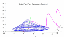
These eigenvectors have several interesting implications. First, the two eigenvalue/eigenvector pairs ([math]\displaystyle{ v_{1} }[/math] and [math]\displaystyle{ v_{2} }[/math]) are responsible for the steady outward slide that occurs in the main disk of the attractor. The last eigenvalue/eigenvector pair is attracting along an axis that runs through the center of the manifold and accounts for the z motion that occurs within the attractor. This effect is roughly demonstrated with the figure below.

The figure examines the central fixed point eigenvectors. The blue line corresponds to the standard Rössler attractor generated with [math]\displaystyle{ a=0.2 }[/math], [math]\displaystyle{ b=0.2 }[/math], and [math]\displaystyle{ c=5.7 }[/math]. The red dot in the center of this attractor is [math]\displaystyle{ FP_{1} }[/math]. The red line intersecting that fixed point is an illustration of the repulsing plane generated by [math]\displaystyle{ v_{1} }[/math] and [math]\displaystyle{ v_{2} }[/math]. The green line is an illustration of the attracting [math]\displaystyle{ v_{3} }[/math]. The magenta line is generated by stepping backwards through time from a point on the attracting eigenvector which is slightly above [math]\displaystyle{ FP_{1} }[/math] – it illustrates the behavior of points that become completely dominated by that vector. Note that the magenta line nearly touches the plane of the attractor before being pulled upwards into the fixed point; this suggests that the general appearance and behavior of the Rössler attractor is largely a product of the interaction between the attracting [math]\displaystyle{ v_{3} }[/math] and the repelling [math]\displaystyle{ v_{1} }[/math] and [math]\displaystyle{ v_{2} }[/math] plane. Specifically it implies that a sequence generated from the Rössler equations will begin to loop around [math]\displaystyle{ FP_{1} }[/math], start being pulled upwards into the [math]\displaystyle{ v_{3} }[/math] vector, creating the upward arm of a curve that bends slightly inward toward the vector before being pushed outward again as it is pulled back towards the repelling plane.

For the outlier fixed point, Rössler's original parameter values of [math]\displaystyle{ a=0.2 }[/math], [math]\displaystyle{ b=0.2 }[/math], and [math]\displaystyle{ c=5.7 }[/math] yield eigenvalues of:

[math]\displaystyle{ \lambda_{1}= -0.0000046 + 5.4280259i }[/math]

[math]\displaystyle{ \lambda_{2}= -0.0000046 - 5.4280259i }[/math]

[math]\displaystyle{ \lambda_{3}= 0.1929830 }[/math]

The eigenvectors corresponding to these eigenvalues are:

[math]\displaystyle{ v_{1}= \begin{pmatrix}0.0002422 + 0.1872055i \\ 0.0344403 - 0.0013136i \\ 0.9817159 \\\end{pmatrix} }[/math]

[math]\displaystyle{ v_{2}= \begin{pmatrix}0.0002422 - 0.1872055i \\ 0.0344403 + 0.0013136i \\ 0.9817159 \\\end{pmatrix} }[/math]

[math]\displaystyle{ v_{3}= \begin{pmatrix}0.0049651 \\ -0.7075770 \\ 0.7066188 \\\end{pmatrix} }[/math]

Although these eigenvalues and eigenvectors exist in the Rössler attractor, their influence is confined to iterations of the Rössler system whose initial conditions are in the general vicinity of this outlier fixed point. Except in those cases where the initial conditions lie on the attracting plane generated by [math]\displaystyle{ \lambda_{1} }[/math] and [math]\displaystyle{ \lambda_{2} }[/math], this influence effectively involves pushing the resulting system towards the general Rössler attractor. As the resulting sequence approaches the central fixed point and the attractor itself, the influence of this distant fixed point (and its eigenvectors) will wane.

Poincaré map

Poincaré map for Rössler attractor with [math]\displaystyle{ a=0.1 }[/math], [math]\displaystyle{ b=0.1 }[/math], [math]\displaystyle{ c=14 }[/math]

The Poincaré map is constructed by plotting the value of the function every time it passes through a set plane in a specific direction. An example would be plotting the [math]\displaystyle{ y, z }[/math] value every time it passes through the [math]\displaystyle{ x = 0 }[/math] plane where [math]\displaystyle{ x }[/math] is changing from negative to positive, commonly done when studying the Lorenz attractor. In the case of the Rössler attractor, the [math]\displaystyle{ x = 0 }[/math] plane is uninteresting, as the map always crosses the [math]\displaystyle{ x = 0 }[/math] plane at [math]\displaystyle{ z = 0 }[/math] due to the nature of the Rössler equations. In the [math]\displaystyle{ x=0.1 }[/math] plane for [math]\displaystyle{ a=0.1 }[/math], [math]\displaystyle{ b=0.1 }[/math], [math]\displaystyle{ c=14 }[/math], the Poincaré map shows the upswing in [math]\displaystyle{ z }[/math] values as [math]\displaystyle{ x }[/math] increases, as is to be expected due to the upswing and twist section of the Rössler plot. The number of points in this specific Poincaré plot is infinite, but when a different [math]\displaystyle{ c }[/math] value is used, the number of points can vary. For example, with a [math]\displaystyle{ c }[/math] value of 4, there is only one point on the Poincaré map, because the function yields a periodic orbit of period one, or if the [math]\displaystyle{ c }[/math] value is set to 12.8, there would be six points corresponding to a period six orbit.

Lorenz map

The Lorenz map is the relation between successive maxima of a coordinate in a trajectory. Consider a trajectory on the attractor, and let [math]\displaystyle{ x_{max}(n) }[/math] be the n-th maximum of its x-coordinate. Then [math]\displaystyle{ x_{max}(n) }[/math]-[math]\displaystyle{ x_{max}(n+1) }[/math] scatterplot is almost a curve, meaning that knowing [math]\displaystyle{ x_{max}(n) }[/math] one can almost exactly predict [math]\displaystyle{ x_{max}(n+1) }[/math].

Lorenz map for Rössler attractor with a = 0.2, b = 0.2, c = 5.

Mapping local maxima

[math]\displaystyle{ Z_n }[/math] vs. [math]\displaystyle{ Z_{n+1} }[/math]

In the original paper on the Lorenz Attractor, Edward Lorenz analyzed the local maxima of [math]\displaystyle{ z }[/math] against the immediately preceding local maxima. When visualized, the plot resembled the tent map, implying that similar analysis can be used between the map and attractor. For the Rössler attractor, when the [math]\displaystyle{ z_n }[/math] local maximum is plotted against the next local [math]\displaystyle{ z }[/math] maximum, [math]\displaystyle{ z_{n+1} }[/math], the resulting plot (shown here for [math]\displaystyle{ a=0.2 }[/math], [math]\displaystyle{ b=0.2 }[/math], [math]\displaystyle{ c=5.7 }[/math]) is unimodal, resembling a skewed Hénon map. Knowing that the Rössler attractor can be used to create a pseudo 1-d map, it then follows to use similar analysis methods. The bifurcation diagram is a particularly useful analysis method.

Variation of parameters

Rössler attractor's behavior is largely a factor of the values of its constant parameters [math]\displaystyle{ a }[/math], [math]\displaystyle{ b }[/math], and [math]\displaystyle{ c }[/math]. In general, varying each parameter has a comparable effect by causing the system to converge toward a periodic orbit, fixed point, or escape towards infinity, however the specific ranges and behaviors induced vary substantially for each parameter. Periodic orbits, or "unit cycles," of the Rössler system are defined by the number of loops around the central point that occur before the loops series begins to repeat itself.

Bifurcation diagrams are a common tool for analyzing the behavior of dynamical systems, of which the Rössler attractor is one. They are created by running the equations of the system, holding all but one of the variables constant and varying the last one. Then, a graph is plotted of the points that a particular value for the changed variable visits after transient factors have been neutralised. Chaotic regions are indicated by filled-in regions of the plot.

Varying a

Here, [math]\displaystyle{ b }[/math] is fixed at 0.2, [math]\displaystyle{ c }[/math] is fixed at 5.7 and [math]\displaystyle{ a }[/math] changes. Numerical examination of the attractor's behavior over changing [math]\displaystyle{ a }[/math] suggests it has a disproportional influence over the attractor's behavior. The results of the analysis are:

• [math]\displaystyle{ a \leq 0 }[/math]: Converges to the centrally located fixed point
• [math]\displaystyle{ a = 0.1 }[/math]: Unit cycle of period 1
• [math]\displaystyle{ a = 0.2 }[/math]: Standard parameter value selected by Rössler, chaotic
• [math]\displaystyle{ a = 0.3 }[/math]: Chaotic attractor, significantly more Möbius strip-like (folding over itself).
• [math]\displaystyle{ a = 0.35 }[/math]: Similar to .3, but increasingly chaotic
• [math]\displaystyle{ a = 0.38 }[/math]: Similar to .35, but increasingly chaotic.

Varying b

Bifurcation diagram for the Rössler attractor for varying [math]\displaystyle{ b }[/math]

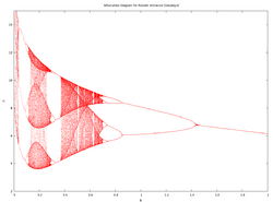
Here, [math]\displaystyle{ a }[/math] is fixed at 0.2, [math]\displaystyle{ c }[/math] is fixed at 5.7 and [math]\displaystyle{ b }[/math] changes. As shown in the accompanying diagram, as [math]\displaystyle{ b }[/math] approaches 0 the attractor approaches infinity (note the upswing for very small values of [math]\displaystyle{ b }[/math]. Comparative to the other parameters, varying [math]\displaystyle{ b }[/math] generates a greater range when period-3 and period-6 orbits will occur. In contrast to [math]\displaystyle{ a }[/math] and [math]\displaystyle{ c }[/math], higher values of [math]\displaystyle{ b }[/math] converge to period-1, not to a chaotic state.

Varying c

File:RosslerVaryC.svg Here, [math]\displaystyle{ a = b = 0.1 }[/math] and [math]\displaystyle{ c }[/math] changes. The bifurcation diagram reveals that low values of [math]\displaystyle{ c }[/math] are periodic, but quickly become chaotic as [math]\displaystyle{ c }[/math] increases. This pattern repeats itself as [math]\displaystyle{ c }[/math] increases – there are sections of periodicity interspersed with periods of chaos, and the trend is towards higher-period orbits as [math]\displaystyle{ c }[/math] increases. For example, the period one orbit only appears for values of [math]\displaystyle{ c }[/math] around 4 and is never found again in the bifurcation diagram. The same phenomenon is seen with period three; until [math]\displaystyle{ c=12 }[/math], period three orbits can be found, but thereafter, they do not appear.

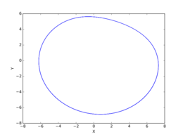
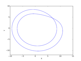
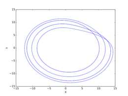
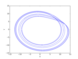
A graphical illustration of the changing attractor over a range of [math]\displaystyle{ c }[/math] values illustrates the general behavior seen for all of these parameter analyses – the frequent transitions between periodicity and aperiodicity.

Varying c

c = 4, period 1

c = 6, period 2

c = 8.5, period 4

c = 8.7, period 8

c = 9, chaotic

c = 12, period 3

c = 12.6, period 6

c = 13, chaotic

Error creating thumbnail: limit.sh: timed out executing command "convert -background "#ffffff00" -thumbnail 260x195\! '/tmp/svg_ce44126f759dc58088d877fb/RosslerC18.svg' PNG:'/tmp/transform_52dc477f1fc6.png'"

c = 18, chaotic

c = 15.4, period 5

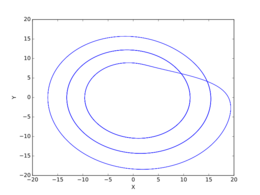
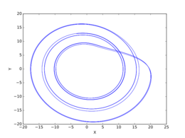
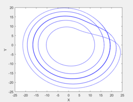
The above set of images illustrates the variations in the post-transient Rössler system as [math]\displaystyle{ c }[/math] is varied over a range of values. These images were generated with [math]\displaystyle{ a=b=.1 }[/math].

• [math]\displaystyle{ c = 4 }[/math], period-1 orbit.
• [math]\displaystyle{ c = 6 }[/math], period-2 orbit.
• [math]\displaystyle{ c = 8.5 }[/math], period-4 orbit.
• [math]\displaystyle{ c = 8.7 }[/math], period-8 orbit.
• [math]\displaystyle{ c = 9 }[/math], sparse chaotic attractor.
• [math]\displaystyle{ c = 12 }[/math], period-3 orbit.
• [math]\displaystyle{ c = 12.6 }[/math], period-6 orbit.
• [math]\displaystyle{ c = 13 }[/math], sparse chaotic attractor.
• [math]\displaystyle{ c = 15.4 }[/math], period-5 orbit.
• [math]\displaystyle{ c = 18 }[/math], filled-in chaotic attractor.

Periodic orbits

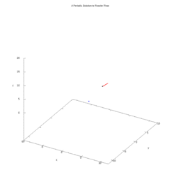
The attractor is filled densely with periodic orbits: solutions for which there exists a nonzero value of [math]\displaystyle{ T }[/math] such that [math]\displaystyle{ \vec{x}(t+T) = \vec{x}(t) }[/math]. These interesting solutions can be numerically derived using Newton's method. Periodic orbits are the roots of the function [math]\displaystyle{ \Phi_t - Id }[/math], where [math]\displaystyle{ \Phi_t }[/math] is the evolution by time [math]\displaystyle{ t }[/math] and [math]\displaystyle{ Id }[/math] is the identity. As the majority of the dynamics occurs in the x-y plane, the periodic orbits can then be classified by their winding number around the central equilibrium after projection.

Table of Periodic Orbits by Winding Number k

k=1

k = 2

k = 3

Time is not to scale. The original parameters (a,b,c) = (0.2,0.2,5.7) were used.

It seems from numerical experimentation that there is a unique periodic orbit for all positive winding numbers. This lack of degeneracy likely stems from the problem's lack of symmetry. The attractor can be dissected into easier to digest invariant manifolds: 1D periodic orbits and the 2D stable and unstable manifolds of periodic orbits. These invariant manifolds are a natural skeleton of the attractor, just as rational numbers are to the real numbers.

For the purposes of dynamical systems theory, one might be interested in topological invariants of these manifolds. Periodic orbits are copies of [math]\displaystyle{ S^1 }[/math] embedded in [math]\displaystyle{ \mathbb{R}^3 }[/math], so their topological properties can be understood with knot theory. The periodic orbits with winding numbers 1 and 2 form a Hopf link, showing that no diffeomorphism can separate these orbits.

Links to other topics

The banding evident in the Rössler attractor is similar to a Cantor set rotated about its midpoint. Additionally, the half-twist that occurs in the Rössler attractor only affects a part of the attractor. Rössler showed that his attractor was in fact the combination of a "normal band" and a Möbius strip.

External links

• Flash Animation using PovRay
• Lorenz and Rössler attractors – Java animation
• 3D Attractors: Mac program to visualize and explore the Rössler and Lorenz attractors in 3 dimensions
• Rössler attractor in Scholarpedia
• Rössler Attractor : Numerical interactive experiment in 3D - experiences.math.cnrs.fr- (javascript/webgl)

References

- ↑ 1.0 1.1 1.2 "An Equation for Continuous Chaos", Physics Letters 57A (5): 397–398, 1976, doi:10.1016/0375-9601(76)90101-8, Bibcode: 1976PhLA...57..397R.
- ↑ "An Equation for Hyperchaos", Physics Letters 71A (2,3): 155–157, 1979, doi:10.1016/0375-9601(79)90150-6, Bibcode: 1979PhLA...71..155R.
- ↑ 3.0 3.1 "12.3 The Rössler Attractor", Chaos and Fractals: New Frontiers of Science, Springer, 2004, pp. 636–646.
- ↑ Rössler, Otto E. (1983-07-01). "The Chaotic Hierarchy" (in en). Zeitschrift für Naturforschung A 38 (7): 788–801. doi:10.1515/zna-1983-0714. ISSN 1865-7109. https://www.degruyter.com/document/doi/10.1515/zna-1983-0714/html.
- ↑ Letellier, C.; P. Dutertre; B. Maheu (1995). "Unstable periodic orbits and templates of the Rössler system: toward a systematic topological characterization". Chaos 5 (1): 272–281. doi:10.1063/1.166076. PMID 12780181. Bibcode: 1995Chaos...5..271L.
- ↑ Letellier, C.; V. Messager (2010). "Influences on Otto E. Rössler's earliest paper on chaos". International Journal of Bifurcation and Chaos 20 (11): 3585–3616. doi:10.1142/s0218127410027854. Bibcode: 2010IJBC...20.3585L.
- ↑ Martines-Arano, H.; García-Pérez, B.E.; Vidales-Hurtado, M.A.; Trejo-Valdez, M.; Hernández-Gómez, L.H.; Torres-Torres, C. (2019). "Chaotic Signatures Exhibited by Plasmonic Effects in Au Nanoparticles with Cells.". Sensors 19 (21): 4728. doi:10.3390/s19214728. PMID 31683534. Bibcode: 2019Senso..19.4728M.
- ↑ Olsen, Lars Folke; Degn, Hans (May 1985). "Chaos in biological systems" (in en). Quarterly Reviews of Biophysics 18 (2): 165–225. doi:10.1017/S0033583500005175. ISSN 1469-8994. https://www.cambridge.org/core/journals/quarterly-reviews-of-biophysics/article/abs/chaos-in-biological-systems/C6B4137C85752FDE43A5DD3F4E615A24.
- ↑ "Deterministic nonperiodic flow", J. Atmos. Sci. 20 (2): 130–141, 1963, doi:10.1175/1520-0469(1963)020<0130:DNF>2.0.CO;2, Bibcode: 1963JAtS...20..130L.
- ↑ Rössler, Otto E. (1976). "Chaotic behavior in simple reaction system". Zeitschrift für Naturforschung A 31 (3–4): 259–264. doi:10.1515/zna-1976-3-408. Bibcode: 1976ZNatA..31..259R. http://www.atomosyd.net/spip.php?article6.