Lorenz system
This article may be too technical for most readers to understand. Please help improve it to make it understandable to non-experts, without removing the technical details. (December 2023) (Learn how and when to remove this template message) |

The Lorenz system is a set of three ordinary differential equations, first developed by the meteorologist Edward Lorenz while studying atmospheric convection. It is a classic example of a system that can exhibit chaotic behavior, meaning its output can be highly sensitive to small changes in its starting conditions.
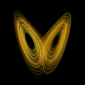
For certain values of its parameters, the system's solutions form a complex, looping pattern known as the Lorenz attractor. The shape of this attractor, when graphed, is famously said to resemble a butterfly. The system's extreme sensitivity to initial conditions gave rise to the popular concept of the butterfly effect—the idea that a small event, like the flap of a butterfly's wings, could ultimately alter large-scale weather patterns. While the system is deterministic—its future behavior is fully determined by its initial conditions—its chaotic nature makes long-term prediction practically impossible.
Although the system is deterministic, (its future behavior is fully determined by its initial conditions) its dynamics depend strongly on the choice of parameters. For some ranges of parameters, the system is predictable: trajectories settle into fixed points or simple periodic orbits, making the long-term behavior easy to describe. For example, when ρ < 1, all solutions converge to the origin, and for certain moderate values of ρ, σ, and β, solutions converge to symmetric steady states.
In contrast, for other parameter ranges, the system becomes chaotic. With the well-known parameters σ = 10, ρ = 28, and β = 8/3, the solutions never settle down but instead trace out the butterfly-shaped Lorenz attractor. In this regime, small differences in initial conditions grow exponentially, so long-term prediction is practically impossible.
Overview
In 1963, Edward Lorenz developed the system as a simplified mathematical model for atmospheric convection.[1] He was attempting to model the way air moves when heated from below and cooled from above. The model describes how three key properties of this system change over time:
- x is proportional to the intensity of the convection (the rate of fluid flow).
- y is proportional to the temperature difference between the rising and falling air currents.
- z is proportional to the distortion of the vertical temperature profile from a linear one.
The model was developed with the assistance of Ellen Fetter, who performed the numerical simulations and created the figures,[1] and Margaret Hamilton, who aided in the initial computations.[2] The behavior of these three variables is governed by the following equations:
The constants σ, ρ, and β are parameters representing physical properties of the system: σ is the Prandtl number, ρ is the Rayleigh number, and β relates to the physical dimensions of the fluid layer itself.[3]
From a technical standpoint, the Lorenz system is nonlinear, aperiodic, three-dimensional, and deterministic. While originally for weather, the equations have since been found to model behavior in a wide variety of systems, including lasers,[4] dynamos,[5] electric circuits,[6] and even some chemical reactions.[7] The Lorenz equations have been the subject of hundreds of research articles and at least one book-length study.[3]
Analysis
One normally assumes that the parameters σ, ρ, and β are positive. Lorenz used the values σ = 10, ρ = 28, and β = 8/3. The system exhibits chaotic behavior for these (and nearby) values.[8]
If ρ < 1 then there is only one equilibrium point, which is at the origin. This point corresponds to no convection. All orbits converge to the origin, which is a global attractor, when ρ < 1.[9]
A pitchfork bifurcation occurs at ρ = 1, and for ρ > 1 two additional critical points appear at These correspond to steady convection. This pair of equilibrium points is stable only if
which can hold only for positive ρ if σ > β + 1. At the critical value, both equilibrium points lose stability through a subcritical Hopf bifurcation.[10]
When ρ = 28, σ = 10, and β = 8/3, the Lorenz system has chaotic solutions (but not all solutions are chaotic). Almost all initial points will tend to an invariant set – the Lorenz attractor – a strange attractor, a fractal, and a self-excited attractor with respect to all three equilibria. Its Hausdorff dimension is estimated from above by the Lyapunov dimension (Kaplan-Yorke dimension) as 2.06±0.01,[11] and the correlation dimension is estimated to be 2.05±0.01.[12] The exact Lyapunov dimension formula of the global attractor can be found analytically under classical restrictions on the parameters:[13][11][14]
The Lorenz attractor is difficult to analyze, but the action of the differential equation on the attractor is described by a fairly simple geometric model.[15] Proving that this is indeed the case is the fourteenth problem on the list of Smale's problems. This problem was the first one to be resolved, by Warwick Tucker in 2002.[16]
For other values of ρ, the system displays knotted periodic orbits. For example, with ρ = 99.96 it becomes a T(3,2) torus knot.
| Example solutions of the Lorenz system for different values of ρ | |
|---|---|
| Image:Lorenz Ro14 20 41 20-200px.png | Image:Lorenz Ro13-200px.png |
| ρ = 14, σ = 10, β = 8/3 (Enlarge) | ρ = 13, σ = 10, β = 8/3 (Enlarge) |
| Image:Lorenz Ro15-200px.png | Image:Lorenz Ro28-200px.png |
| ρ = 15, σ = 10, β = 8/3 (Enlarge) | ρ = 28, σ = 10, β = 8/3 (Enlarge) |
| For small values of ρ, the system is stable and evolves to one of two fixed point attractors. When ρ > 24.74, the fixed points become repulsors and the trajectory is repelled by them in a very complex way. | |
| Sensitive dependence on the initial condition | ||
|---|---|---|
| Time t = 1 (Enlarge) | Time t = 2 (Enlarge) | Time t = 3 (Enlarge) |
| Image:Lorenz caos1-175.png | Image:Lorenz caos2-175.png | Image:Lorenz caos3-175.png |
| These figures — made using ρ = 28, σ = 10, and β = 8/3 — show three time segments of the 3-D evolution of two trajectories (one in blue, the other in yellow) in the Lorenz attractor starting at two initial points that differ only by 10−5 in the x-coordinate. Initially, the two trajectories seem coincident (only the yellow one can be seen, as it is drawn over the blue one) but, after some time, the divergence is obvious. | ||
| Divergence of nearby trajectories. |
|---|
 |
| The parameters are: , , and . Significant divergence is seen at around , beyond which the trajectories become uncorrelated. The full-sized graphic can be accessed here. |
Connection to tent map

In Figure 4 of his paper,[1] Lorenz plotted the relative maximum value in the z direction achieved by the system against the previous relative maximum in the z direction. This procedure later became known as a Lorenz map (not to be confused with a Poincaré plot, which plots the intersections of a trajectory with a prescribed surface). The resulting plot has a shape very similar to the tent map. Lorenz also found that when the maximum z value is above a certain cut-off, the system will switch to the next lobe. Combining this with the chaos known to be exhibited by the tent map, he showed that the system switches between the two lobes chaotically.
Generalized Lorenz system
Over the past several years, a series of papers regarding high-dimensional Lorenz models have yielded a generalized Lorenz model,[17] which can be simplified into the classical Lorenz model for three state variables or the following five-dimensional Lorenz model for five state variables:[18]
A choice of the parameter has been applied to be consistent with the choice of the other parameters. See details in.[17][18]
Simulations

Julia simulation
using Plots
# define the Lorenz attractor
@kwdef mutable struct Lorenz
    dt::Float64 = 0.02
    σ::Float64 = 10
    ρ::Float64 = 28
    β::Float64 = 8/3
    x::Float64 = 2
    y::Float64 = 1
    z::Float64 = 1
end

function step!(l::Lorenz)
    dx = l.σ * (l.y - l.x)
    dy = l.x * (l.ρ - l.z) - l.y
    dz = l.x * l.y - l.β * l.z
    l.x += l.dt * dx
    l.y += l.dt * dy
    l.z += l.dt * dz
end

attractor = Lorenz()

# initialize a 3D plot with 1 empty series
plt = plot3d(
    1,
    xlim = (-30, 30),
    ylim = (-30, 30),
    zlim = (0, 60),
    title = "Lorenz Attractor",
    marker = 2,
)

# build an animated gif by pushing new points to the plot, saving every 10th frame
@gif for i=1:1500
    step!(attractor)
    push!(plt, attractor.x, attractor.y, attractor.z)
end every 10
Maple simulation
deq := [diff(x(t), t) = 10*(y(t) - x(t)), diff(y(t), t) = 28*x(t) - y(t) - x(t)*z(t), diff(z(t), t) = x(t)*y(t) - 8/3*z(t)]:
with(DEtools):
DEplot3d(deq, {x(t), y(t), z(t)}, t = 0 .. 100, x(0) = 10, y(0) = 10, z(0) = 10, stepsize = 0.01, x = -20 .. 20, y = -25 .. 25, z = 0 .. 50, linecolour = sin(t*Pi/3), thickness = 1, orientation = [-40, 80], title = `Lorenz Chaotic Attractor`);
Maxima simulation
[sigma, rho, beta]: [10, 28, 8/3]$
eq: [sigma*(y-x), x*(rho-z)-y, x*y-beta*z]$
sol: rk(eq, [x, y, z], [1, 0, 0], [t, 0, 50, 1/100])$
len: length(sol)$
x: makelist(sol[k][2], k, len)$
y: makelist(sol[k][3], k, len)$
z: makelist(sol[k][4], k, len)$
draw3d(points_joined=true, point_type=-1, points(x, y, z), proportional_axes=xyz)$
MATLAB simulation
% Solve over time interval [0,100] with initial conditions [1,1,1]
% ''f'' is set of differential equations
% ''a'' is array containing x, y, and z variables
% ''t'' is time variable

sigma = 10;
beta = 8/3;
rho = 28;
f = @(t,a) [-sigma*a(1) + sigma*a(2); rho*a(1) - a(2) - a(1)*a(3); -beta*a(3) + a(1)*a(2)];
[t,a] = ode45(f,[0 100],[1 1 1]);     % Runge-Kutta 4th/5th order ODE solver
plot3(a(:,1),a(:,2),a(:,3))
Mathematica simulation
Standard way:
tend = 50;
eq = {x'[t] == σ (y[t] - x[t]),
      y'[t] == x[t] (ρ - z[t]) - y[t],
      z'[t] == x[t] y[t] - β z[t]};
init = {x[0] == 10, y[0] == 10, z[0] == 10};
pars = {σ->10, ρ->28, β->8/3};
{xs, ys, zs} =
  NDSolveValue[{eq /. pars, init}, {x, y, z}, {t, 0, tend}];
ParametricPlot3D[{xs[t], ys[t], zs[t]}, {t, 0, tend}]
Less verbose:
lorenz = NonlinearStateSpaceModel[{{σ (y - x), x (ρ - z) - y, x y - β z}, {}}, {x, y, z}, {σ, ρ, β}];
soln[t_] = StateResponse[{lorenz, {10, 10, 10}}, {10, 28, 8/3}, {t, 0, 50}];
ParametricPlot3D[soln[t], {t, 0, 50}]
R simulation
library(deSolve)
library(plotly)
# parameters
prm <- list(sigma = 10, rho = 28, beta = 8/3)
# initial values
varini <- c(
  X = 1,
  Y = 1,
  Z = 1
)

Lorenz <- function (t, vars, prm) {
  with(as.list(vars), {
    dX <- prm$sigma*(Y - X)
    dY <- X*(prm$rho - Z) - Y
    dZ <- X*Y - prm$beta*Z
    return(list(c(dX, dY, dZ)))
   })
}

times <- seq(from = 0, to = 100, by = 0.01)
# call ode solver
out <- ode(y = varini, times = times, func = Lorenz,
           parms = prm)

# to assign color to points
gfill <- function (repArr, long) {
  rep(repArr, ceiling(long/length(repArr)))[1:long]
}

dout <- as.data.frame(out)

dout$color <- gfill(rainbow(10), nrow(dout))

# Graphics production with Plotly:
plot_ly(
  data=dout, x = ~X, y = ~Y, z = ~Z,
  type = 'scatter3d', mode = 'lines',
  opacity = 1, line = list(width = 6, color = ~color, reverscale = FALSE)
)

SageMath simulation
We try to solve this system of equations for , , , with initial conditions , , .
# we solve the Lorenz system of the differential equations.
# Runge-Kutta's method y_{n+1}= y_n + h*(k_1 + 2*k_2+2*k_3+k_4)/6; x_{n+1}=x_n+h
# k_1=f(x_n,y_n), k_2=f(x_n+h/2, y_n+hk_1/2), k_3=f(x_n+h/2, y_n+hk_2/2), k_4=f(x_n+h, y_n+hk_3)
# differential equation
def Runge_Kutta(f,v,a,b,h,n):
    tlist = [a+i*h for i in range(n+1)]
    y = [[0,0,0] for _ in range(n+1)]
    # Taking length of f (number of equations).
    m=len(f)
    # Number of variables in v.
    vm=len(v)
    if m!=vm:
        return("error, number of equations is not equal with the number of variables.")
    for r in range(vm):
        y[0][r]=b[r]
    # making a vector and component will be a list
    # main part of the algorithm
    k1=[0 for _ in range(m)]
    k2=[0 for _ in range(m)]
    k3=[0 for _ in range(m)]
    k4=[0 for _ in range(m)]
    for i in range(1,n+1): # for each t_i, i=1, ... , n
        # k1=h*f(t_{i-1},x_1(t_{i-1}),...,x_m(t_{i-1}))
        for j in range(m): # for each f_{j+1}, j=0, ... , m-1
            k1[j]=f[j].subs(t==tlist[i-1])
            for r in range(vm):
                k1[j]=k1[j].subs(v[r]==y[i-1][r])
            k1[j]=h*k1[j]
        for j in range(m): # k2=h*f(t_{i-1}+h/2,x_1(t_{i-1})+k1/2,...,x_m(t_{i-1}+k1/2))
            k2[j]=f[j].subs(t==tlist[i-1]+h/2)
            for r in range(vm):
                k2[j]=k2[j].subs(v[r]==y[i-1][r]+k1[r]/2)
            k2[j]=h*k2[j]
        for j in range(m): # k3=h*f(t_{i-1}+h/2,x_1(t_{i-1})+k2/2,...,x_m(t_{i-1})+k2/2)
            k3[j]=f[j].subs(t==tlist[i-1]+h/2)
            for r in range(vm):
                k3[j]=k3[j].subs(v[r]==y[i-1][r]+k2[r]/2)
            k3[j]=h*k3[j]
        for j in range(m): # k4=h*f(t_{i-1}+h,x_1(t_{i-1})+k3,...,x_m(t_{i-1})+k3)
            k4[j]=f[j].subs(t==tlist[i-1]+h)
            for r in range(vm):
                k4[j]=k4[j].subs(v[r]==y[i-1][r]+k3[r])
            k4[j]=h*k4[j]
        for j in range(m): # Now x_j(t_i)=x_j(t_{i-1})+(k1+2k2+2k3+k4)/6
            y[i][j]=y[i-1][j]+(k1[j]+2*k2[j]+2*k3[j]+k4[j])/6
    return(tlist,y)

# (Figure 1) Here, we plot the solutions of the Lorenz ODE system.
a=0.0 # t_0
b=[0.0,.50,0.0] # x_1(t_0), ... , x_m(t_0)
t=var('t')
x = var('x', n=3, latex_name='x')
v=[x[ii] for ii in range(3)]
f= [10*(x1-x0),x0*(28-x2)-x1,x0*x1-(8/3)*x2];
n=1600
h=0.0125
tlist,y=Runge_Kutta(f,v,a,b,h,n)
#print(tlist)
#print(y)
T=point3d(y[i][0],y[i][1],y[i][2 for i in range(n)], color='red')
S=line3d(y[i][0],y[i][1],y[i][2 for i in range(n)], color='red')
show(T+S)

# (Figure 2) Here, we plot every y1, y2, and y3 in terms of time.
a=0.0 # t_0
b=[0.0,.50,0.0] # x_1(t_0), ... , x_m(t_0)
t=var('t')
x = var('x', n=3, latex_name='x')
v=[x[ii] for ii in range(3)]
Lorenz= [10*(x1-x0),x0*(28-x2)-x1,x0*x1-(8/3)*x2];
n=100
h=0.1
tlist,y=Runge_Kutta(Lorenz,v,a,b,h,n)
#Runge_Kutta(f,v,0,b,h,n)
#print(tlist)
#print(y)
P1=list_plot(tlist[i],y[i][0 for i in range(n)], plotjoined=True, color='red');
P2=list_plot(tlist[i],y[i][1 for i in range(n)], plotjoined=True, color='green');
P3=list_plot(tlist[i],y[i][2 for i in range(n)], plotjoined=True, color='yellow');
show(P1+P2+P3)

# (Figure 3) Here, we plot the y and x or equivalently y2 and y1
a=0.0 # t_0
b=[0.0,.50,0.0] # x_1(t_0), ... , x_m(t_0)
t=var('t')
x = var('x', n=3, latex_name='x')
v=[x[ii] for ii in range(3)]
f= [10*(x1-x0),x0*(28-x2)-x1,x0*x1-(8/3)*x2];
n=800
h=0.025
tlist,y=Runge_Kutta(f,v,a,b,h,n)
vv=y[i][0],y[i][1 for i in range(n)];
#print(tlist)
#print(y)
T=points(vv, rgbcolor=(0.2,0.6, 0.1), pointsize=10)
S=line(vv,rgbcolor=(0.2,0.6, 0.1))
show(T+S)

# (Figure 4) Here, we plot the z and x or equivalently y3 and y1
a=0.0 # t_0
b=[0.0,.50,0.0] # x_1(t_0), ... , x_m(t_0)
t=var('t')
x = var('x', n=3, latex_name='x')
v=[x[ii] for ii in range(3)]
f= [10*(x1-x0),x0*(28-x2)-x1,x0*x1-(8/3)*x2];
n=800
h=0.025
tlist,y=Runge_Kutta(f,v,a,b,h,n)
vv=y[i][0],y[i][2 for i in range(n)];
#print(tlist)
#print(y)
T=points(vv, rgbcolor=(0.2,0.6, 0.1), pointsize=10)
S=line(vv,rgbcolor=(0.2,0.6, 0.1))
show(T+S)

# (Figure 5) Here, we plot the z and x or equivalently y3 and y2
a=0.0 # t_0
b=[0.0,.50,0.0] # x_1(t_0), ... , x_m(t_0)
t=var('t')
x = var('x', n=3, latex_name='x')
v=[x[ii] for ii in range(3)]
f= [10*(x1-x0),x0*(28-x2)-x1,x0*x1-(8/3)*x2];
n=800
h=0.025
tlist,y=Runge_Kutta(f,v,a,b,h,n)
vv=y[i][1],y[i][2 for i in range(n)];
#print(tlist)
#print(y)
T=points(vv, rgbcolor=(0.2,0.6, 0.1), pointsize=10)
S=line(vv,rgbcolor=(0.2,0.6, 0.1))
show(T+S)
Applications
Model for atmospheric convection
As shown in Lorenz's original paper,[19] the Lorenz system is a reduced version of a larger system studied earlier by Barry Saltzman.[20] The Lorenz equations are derived from the Oberbeck–Boussinesq approximation to the equations describing fluid circulation in a shallow layer of fluid, heated uniformly from below and cooled uniformly from above.[21] This fluid circulation is known as Rayleigh–Bénard convection. The fluid is assumed to circulate in two dimensions (vertical and horizontal) with periodic rectangular boundary conditions.[22]
The partial differential equations modeling the system's stream function and temperature are subjected to a spectral Galerkin approximation: the hydrodynamic fields are expanded in Fourier series, which are then severely truncated to a single term for the stream function and two terms for the temperature. This reduces the model equations to a set of three coupled, nonlinear ordinary differential equations. A detailed derivation may be found, for example, in nonlinear dynamics texts from (Hilborn 2000), Appendix C; (Bergé Pomeau), Appendix D; or Shen (2016),[23] Supplementary Materials.
Model for the nature of chaos and order in the atmosphere
The scientific community accepts that the chaotic features found in low-dimensional Lorenz models could represent features of the Earth's atmosphere,[24][25][26] yielding the statement of “weather is chaotic.” By comparison, based on the concept of attractor coexistence within the generalized Lorenz model[17] and the original Lorenz model,[27][28] Shen and his co-authors proposed a revised view that “weather possesses both chaos and order with distinct predictability”.[26][29] The revised view, which is a build-up of the conventional view, is used to suggest that “the chaotic and regular features found in theoretical Lorenz models could better represent features of the Earth's atmosphere”.
Resolution of Smale's 14th problem
Smale's 14th problem asks, "Do the properties of the Lorenz attractor exhibit that of a strange attractor?". The problem was answered affirmatively by Warwick Tucker in 2002.[16] To prove this result, Tucker used rigorous numerics methods like interval arithmetic and normal forms. First, Tucker defined a cross section that is cut transversely by the flow trajectories. From this, one can define the first-return map , which assigns to each the point where the trajectory of first intersects .
Then the proof is split in three main points that are proved and imply the existence of a strange attractor.[30] The three points are:
- There exists a region invariant under the first-return map, meaning .
- The return map admits a forward invariant cone field.
- Vectors inside this invariant cone field are uniformly expanded by the derivative of the return map.
To prove the first point, we notice that the cross section is cut by two arcs formed by .[30] Tucker covers the location of these two arcs by small rectangles , the union of these rectangles gives . Now, the goal is to prove that for all points in , the flow will bring back the points in , in . To do that, we take a plan below at a distance small, then by taking the center of and using Euler integration method, one can estimate where the flow will bring in which gives us a new point . Then, one can estimate where the points in will be mapped in using Taylor expansion, this gives us a new rectangle centered on . Thus we know that all points in will be mapped in . The goal is to do this method recursively until the flow comes back to and we obtain a rectangle in such that we know that . The problem is that our estimation may become imprecise after several iterations, thus what Tucker does is to split into smaller rectangles and then apply the process recursively. Another problem is that as we are applying this algorithm, the flow becomes more 'horizontal',[30] leading to a dramatic increase in imprecision. To prevent this, the algorithm changes the orientation of the cross sections, becoming either horizontal or vertical.
Gallery
-
 A solution in the Lorenz attractor plotted at high resolution in the xz plane.
 -
 A solution in the Lorenz attractor rendered as an SVG.
 -
An animation showing trajectories of multiple solutions in a Lorenz system.
-
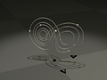 A solution in the Lorenz attractor rendered as a metal wire to show direction and 3D structure.
 -
An animation showing the divergence of nearby solutions to the Lorenz system.
-
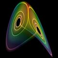 A visualization of the Lorenz attractor near an intermittent cycle.
 -
 Two streamlines in a Lorenz system, from ρ = 0 to ρ = 28 (σ = 10, β = 8/3).
 -
 Animation of a Lorenz System with rho-dependence.
 -
![Animation of the Lorenz attractor in the Brain Dynamics Toolbox.[31]](/wiki/images/thumb/f/f8/Lorenz_Attractor_Brain_Dynamics_Toolbox.gif/120px-Lorenz_Attractor_Brain_Dynamics_Toolbox.gif) Animation of the Lorenz attractor in the Brain Dynamics Toolbox.[31]
Animation of the Lorenz attractor in the Brain Dynamics Toolbox.[31]


.gif)
![Animation of the Lorenz attractor in the Brain Dynamics Toolbox.[31]](/wiki/File:Lorenz_Attractor_Brain_Dynamics_Toolbox.gif)
See also
- Eden's conjecture on the Lyapunov dimension
- Lorenz 96 model
- List of chaotic maps
- Takens' theorem
Notes
- ↑ 1.0 1.1 1.2 (Lorenz 1963)
- ↑ (Lorenz 1960)
- ↑ 3.0 3.1 (Sparrow 1982)
- ↑ (Haken 1975)
- ↑ (Knobloch 1981)
- ↑ (Cuomo Oppenheim)
- ↑ (Poland 1993)
- ↑ (Hirsch Smale), pp. 303–305
- ↑ (Hirsch Smale), pp. 306+307
- ↑ (Hirsch Smale), pp. 307–308
- ↑ 11.0 11.1 Kuznetsov, N.V.; Mokaev, T.N.; Kuznetsova, O.A.; Kudryashova, E.V. (2020). "The Lorenz system: hidden boundary of practical stability and the Lyapunov dimension". Nonlinear Dynamics 102 (2): 713–732. doi:10.1007/s11071-020-05856-4. Bibcode: 2020NonDy.102..713K.
- ↑ (Grassberger Procaccia)
- ↑ (Leonov Kuznetsov)
- ↑ Kuznetsov, Nikolay; Reitmann, Volker (2021). Attractor Dimension Estimates for Dynamical Systems: Theory and Computation. Cham: Springer. https://www.springer.com/gp/book/9783030509866.
- ↑ Guckenheimer, John; Williams, R. F. (1979-12-01). "Structural stability of Lorenz attractors". Publications Mathématiques de l'Institut des Hautes Études Scientifiques 50 (1): 59–72. doi:10.1007/BF02684769. ISSN 0073-8301. http://www.numdam.org/item/PMIHES_1979__50__59_0/.
- ↑ 16.0 16.1 (Tucker 2002)
- ↑ 17.0 17.1 17.2 Shen, Bo-Wen (2019-03-01). "Aggregated Negative Feedback in a Generalized Lorenz Model". International Journal of Bifurcation and Chaos 29 (3): 1950037–1950091. doi:10.1142/S0218127419500378. ISSN 0218-1274. Bibcode: 2019IJBC...2950037S.
- ↑ 18.0 18.1 Shen, Bo-Wen (2014-04-28). "Nonlinear Feedback in a Five-Dimensional Lorenz Model". Journal of the Atmospheric Sciences 71 (5): 1701–1723. doi:10.1175/jas-d-13-0223.1. ISSN 0022-4928. Bibcode: 2014JAtS...71.1701S. http://dx.doi.org/10.1175/jas-d-13-0223.1.
- ↑ (Lorenz 1963)
- ↑ (Saltzman 1962)
- ↑ (Lorenz 1963)
- ↑ (Lorenz 1963)
- ↑ Shen, B.-W. (2015-12-21). "Nonlinear feedback in a six-dimensional Lorenz model: impact of an additional heating term" (in en). Nonlinear Processes in Geophysics 22 (6): 749–764. doi:10.5194/npg-22-749-2015. ISSN 1607-7946. Bibcode: 2015NPGeo..22..749S. https://npg.copernicus.org/articles/22/749/2015/.
- ↑ Ghil, Michael; Read, Peter; Smith, Leonard (2010-07-23). "Geophysical flows as dynamical systems: the influence of Hide's experiments". Astronomy & Geophysics 51 (4): 4.28–4.35. doi:10.1111/j.1468-4004.2010.51428.x. ISSN 1366-8781. Bibcode: 2010A&G....51d..28G. http://dx.doi.org/10.1111/j.1468-4004.2010.51428.x.
- ↑ Read, P. (1993). Application of Chaos to Meteorology and Climate. In The Nature of Chaos; Mullin, T., Ed. Oxford, UK: Oxford Science Publications. pp. 220–260. ISBN 0198539541.
- ↑ 26.0 26.1 Shen, Bo-Wen; Pielke, Roger; Zeng, Xubin; Cui, Jialin; Faghih-Naini, Sara; Paxson, Wei; Kesarkar, Amit; Zeng, Xiping et al. (2022-11-12). "The Dual Nature of Chaos and Order in the Atmosphere" (in en). Atmosphere 13 (11): 1892. doi:10.3390/atmos13111892. ISSN 2073-4433. Bibcode: 2022Atmos..13.1892S.
- ↑ Yorke, James A.; Yorke, Ellen D. (1979-09-01). "Metastable chaos: The transition to sustained chaotic behavior in the Lorenz model" (in en). Journal of Statistical Physics 21 (3): 263–277. doi:10.1007/BF01011469. ISSN 1572-9613. Bibcode: 1979JSP....21..263Y. https://doi.org/10.1007/BF01011469.
- ↑ Shen, Bo-Wen; Pielke, R. A.; Zeng, X.; Baik, J.-J.; Faghih-Naini, S.; Cui, J.; Atlas, R.; Reyes, T. A. L. (2021), Skiadas, Christos H.; Dimotikalis, Yiannis, eds., "Is Weather Chaotic? Coexisting Chaotic and Non-chaotic Attractors within Lorenz Models" (in en), 13th Chaotic Modeling and Simulation International Conference, Springer Proceedings in Complexity (Cham: Springer International Publishing): pp. 805–825, doi:10.1007/978-3-030-70795-8_57, ISBN 978-3-030-70794-1, https://link.springer.com/10.1007/978-3-030-70795-8_57, retrieved 2022-12-22
- ↑ Shen, Bo-Wen; Pielke, Roger A.; Zeng, Xubin; Baik, Jong-Jin; Faghih-Naini, Sara; Cui, Jialin; Atlas, Robert (2021-01-01). "Is Weather Chaotic?: Coexistence of Chaos and Order within a Generalized Lorenz Model" (in EN). Bulletin of the American Meteorological Society 102 (1): E148–E158. doi:10.1175/BAMS-D-19-0165.1. ISSN 0003-0007. Bibcode: 2021BAMS..102E.148S.
- ↑ 30.0 30.1 30.2 (Viana 2000)
- ↑ Heitmann, S., Breakspear, M (2017-2022) Brain Dynamics Toolbox. bdtoolbox.org doi.org/10.5281/zenodo.5625923
References
- Bergé, Pierre; Pomeau, Yves; Vidal, Christian (1984). Order within Chaos: Towards a Deterministic Approach to Turbulence. New York: John Wiley & Sons. ISBN 978-0-471-84967-4.
- Cuomo, Kevin M.; Oppenheim, Alan V. (1993). "Circuit implementation of synchronized chaos with applications to communications". Physical Review Letters 71 (1): 65–68. doi:10.1103/PhysRevLett.71.65. ISSN 0031-9007. PMID 10054374. Bibcode: 1993PhRvL..71...65C.
- Gorman, M.; Widmann, P.J.; Robbins, K.A. (1986). "Nonlinear dynamics of a convection loop: A quantitative comparison of experiment with theory". Physica D 19 (2): 255–267. doi:10.1016/0167-2789(86)90022-9. Bibcode: 1986PhyD...19..255G.
- Grassberger, P.; Procaccia, I. (1983). "Measuring the strangeness of strange attractors". Physica D 9 (1–2): 189–208. doi:10.1016/0167-2789(83)90298-1. Bibcode: 1983PhyD....9..189G.
- Haken, H. (1975). "Analogy between higher instabilities in fluids and lasers". Physics Letters A 53 (1): 77–78. doi:10.1016/0375-9601(75)90353-9. Bibcode: 1975PhLA...53...77H.
- Sauermann, H.; Haken, H. (1963). "Nonlinear Interaction of Laser Modes". Z. Phys. 173 (3): 261–275. doi:10.1007/BF01377828. Bibcode: 1963ZPhy..173..261H.
- Ning, C.Z.; Haken, H. (1990). "Detuned lasers and the complex Lorenz equations: Subcritical and supercritical Hopf bifurcations". Phys. Rev. A 41 (7): 3826–3837. doi:10.1103/PhysRevA.41.3826. PMID 9903557. Bibcode: 1990PhRvA..41.3826N.
- Hemati, N. (1994). "Strange attractors in brushless DC motors". IEEE Transactions on Circuits and Systems I: Fundamental Theory and Applications 41 (1): 40–45. doi:10.1109/81.260218. ISSN 1057-7122. Bibcode: 1994ITCSR..41...40H.
- Hilborn, Robert C. (2000). Chaos and Nonlinear Dynamics: An Introduction for Scientists and Engineers (second ed.). Oxford University Press. ISBN 978-0-19-850723-9.
- Hirsch, Morris W.; Smale, Stephen; Devaney, Robert (2003). Differential Equations, Dynamical Systems, & An Introduction to Chaos (Second ed.). Boston, MA: Academic Press. ISBN 978-0-12-349703-1.
- Knobloch, Edgar (1981). "Chaos in the segmented disc dynamo". Physics Letters A 82 (9): 439–440. doi:10.1016/0375-9601(81)90274-7. Bibcode: 1981PhLA...82..439K.
- Kolář, Miroslav; Gumbs, Godfrey (1992). "Theory for the experimental observation of chaos in a rotating waterwheel". Physical Review A 45 (2): 626–637. doi:10.1103/PhysRevA.45.626. PMID 9907027. Bibcode: 1992PhRvA..45..626K.
- Leonov, G.A.; Kuznetsov, N.V.; Korzhemanova, N.A.; Kusakin, D.V. (2016). "Lyapunov dimension formula for the global attractor of the Lorenz system". Communications in Nonlinear Science and Numerical Simulation 41: 84–103. doi:10.1016/j.cnsns.2016.04.032. Bibcode: 2016CNSNS..41...84L.
- Lorenz, Edward Norton (1963). "Deterministic nonperiodic flow". Journal of the Atmospheric Sciences 20 (2): 130–141. doi:10.1175/1520-0469(1963)020<0130:DNF>2.0.CO;2. Bibcode: 1963JAtS...20..130L.
- Mishra, Aashwin; Sanghi, Sanjeev (2006). "A study of the asymmetric Malkus waterwheel: The biased Lorenz equations". Chaos: An Interdisciplinary Journal of Nonlinear Science 16 (1): 013114. doi:10.1063/1.2154792. PMID 16599745. Bibcode: 2006Chaos..16a3114M.
- Pchelintsev, A.N. (2014). "Numerical and Physical Modeling of the Dynamics of the Lorenz System". Numerical Analysis and Applications 7 (2): 159–167. doi:10.1134/S1995423914020098.
- Poland, Douglas (1993). "Cooperative catalysis and chemical chaos: a chemical model for the Lorenz equations". Physica D 65 (1): 86–99. doi:10.1016/0167-2789(93)90006-M. Bibcode: 1993PhyD...65...86P.
- Saltzman, Barry (1962). "Finite Amplitude Free Convection as an Initial Value Problem—I". Journal of the Atmospheric Sciences 19 (4): 329–341. doi:10.1175/1520-0469(1962)019<0329:FAFCAA>2.0.CO;2. Bibcode: 1962JAtS...19..329S.
- Shen, B.-W. (2015-12-21). "Nonlinear feedback in a six-dimensional Lorenz model: impact of an additional heating term". Nonlinear Processes in Geophysics. 22 (6): 749–764. doi:10.5194/npg-22-749-2015. ISSN 1607-7946.
- Sparrow, Colin (1982). The Lorenz Equations: Bifurcations, Chaos, and Strange Attractors. Springer. Bibcode: 1982lebc.book.....S.
- Tucker, Warwick (2002). "A Rigorous ODE Solver and Smale's 14th Problem". Foundations of Computational Mathematics 2 (1): 53–117. doi:10.1007/s002080010018. https://link.springer.com/content/pdf/10.1007/s002080010018.pdf.
- Tzenov, Stephan (2014). "Strange Attractors Characterizing the Osmotic Instability". arXiv:1406.0979v1 [physics.flu-dyn].
- Viana, Marcelo (2000). "What's new on Lorenz strange attractors?". The Mathematical Intelligencer 22 (3): 6–19. doi:10.1007/BF03025276.
- Lorenz, Edward N. (1960). "The statistical prediction of solutions of dynamic equations.". Symposium on Numerical Weather Prediction in Tokyo. http://eaps4.mit.edu/research/Lorenz/The_Statistical_Prediction_of_Solutions_1962.pdf. Retrieved 2020-09-16.
Further reading
- G.A. Leonov; N.V. Kuznetsov (2015). "On differences and similarities in the analysis of Lorenz, Chen, and Lu systems". Applied Mathematics and Computation 256: 334–343. doi:10.1016/j.amc.2014.12.132.
- Pchelintsev, A.N. (2022). "On a high-precision method for studying attractors of dynamical systems and systems of explosive type". Mathematics 10 (8): 1207. doi:10.3390/math10081207. https://www.mdpi.com/2227-7390/10/8/1207/pdf.
External links
- Hazewinkel, Michiel, ed. (2001), "Lorenz attractor", Encyclopedia of Mathematics, Springer Science+Business Media B.V. / Kluwer Academic Publishers, ISBN 978-1-55608-010-4, https://www.encyclopediaofmath.org/index.php?title=p/l060890
- Weisstein, Eric W.. "Lorenz attractor". http://mathworld.wolfram.com/LorenzAttractor.html.
- Lorenz attractor by Rob Morris, Wolfram Demonstrations Project.
- Lorenz Equation at PlanetMath.org.
- Synchronized Chaos and Private Communications, with Kevin Cuomo. The implementation of Lorenz attractor in an electronic circuit.
- 3D Attractors: Mac program to visualize and explore the Lorenz attractor in 3 dimensions
- Lorenz Attractor implemented in analog electronic
- Lorenz Attractor interactive animation (implemented in Ada with GTK+. Sources & executable)


 |  |
