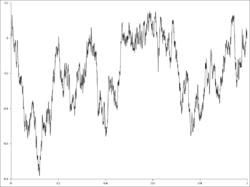
Brownian bridge

Short description: A process in physics

Brownian motion, pinned at both ends. This represents a Brownian bridge.

A Brownian bridge is a continuous-time stochastic process B(t) whose probability distribution is the conditional probability distribution of a standard Wiener process W(t) (a mathematical model of Brownian motion) subject to the condition (when standardized) that W(T) = 0, so that the process is pinned to the same value at both t = 0 and t = T. More precisely:

[math]\displaystyle{ B_t := (W_t\mid W_T=0),\;t \in [0,T] }[/math]

The expected value of the bridge at any t in the interval [0,T] is zero, with variance [math]\displaystyle{ \textstyle\frac{t(T-t)}{T} }[/math], implying that the most uncertainty is in the middle of the bridge, with zero uncertainty at the nodes. The covariance of B(s) and B(t) is [math]\displaystyle{ \min(s,t)-\frac{s\,t}{T} }[/math], or s(T − t)/T if s < t. The increments in a Brownian bridge are not independent.

Relation to other stochastic processes

If W(t) is a standard Wiener process (i.e., for t ≥ 0, W(t) is normally distributed with expected value 0 and variance t, and the increments are stationary and independent), then

[math]\displaystyle{ B(t) = W(t) - \frac{t}{T} W(T)\, }[/math]

is a Brownian bridge for t ∈ [0, T]. It is independent of W(T)

Conversely, if B(t) is a Brownian bridge and Z is a standard normal random variable independent of B, then the process

[math]\displaystyle{ W(t) = B(t) + tZ\, }[/math]

is a Wiener process for t ∈ [0, 1]. More generally, a Wiener process W(t) for t ∈ [0, T] can be decomposed into

[math]\displaystyle{ W(t) = \sqrt{T}B\left(\frac{t}{T}\right) + \frac{t}{\sqrt{T}} Z. }[/math]

Another representation of the Brownian bridge based on the Brownian motion is, for t ∈ [0, T]

[math]\displaystyle{ B(t) = \frac{T-t}{\sqrt T} W\left(\frac{t}{T-t}\right). }[/math]

Conversely, for t ∈ [0, ∞]

[math]\displaystyle{ W(t) = \frac{T+t}{T} B\left(\frac{Tt}{T+t}\right). }[/math]

The Brownian bridge may also be represented as a Fourier series with stochastic coefficients, as

[math]\displaystyle{ B_t = \sum_{k=1}^\infty Z_k \frac{\sqrt{2 T} \sin(k \pi t / T)}{k \pi} }[/math]

where [math]\displaystyle{ Z_1, Z_2, \ldots }[/math] are independent identically distributed standard normal random variables (see the Karhunen–Loève theorem).

A Brownian bridge is the result of Donsker's theorem in the area of empirical processes. It is also used in the Kolmogorov–Smirnov test in the area of statistical inference.

Intuitive remarks

A standard Wiener process satisfies W(0) = 0 and is therefore "tied down" to the origin, but other points are not restricted. In a Brownian bridge process on the other hand, not only is B(0) = 0 but we also require that B(T) = 0, that is the process is "tied down" at t = T as well. Just as a literal bridge is supported by pylons at both ends, a Brownian Bridge is required to satisfy conditions at both ends of the interval [0,T]. (In a slight generalization, one sometimes requires B(t₁) = a and B(t₂) = b where t₁, t₂, a and b are known constants.)

Suppose we have generated a number of points W(0), W(1), W(2), W(3), etc. of a Wiener process path by computer simulation. It is now desired to fill in additional points in the interval [0,T], that is to interpolate between the already generated points W(0) and W(T). The solution is to use a Brownian bridge that is required to go through the values W(0) and W(T).

General case

For the general case when B(t₁) = a and B(t₂) = b, the distribution of B at time t ∈ (t₁, t₂) is normal, with mean

[math]\displaystyle{ a + \frac{t-t_1}{t_2-t_1}(b-a) }[/math]

and variance

[math]\displaystyle{ \frac{(t_2-t)(t-t_1)}{t_2-t_1}, }[/math]

and the covariance between B(s) and B(t), with s < t is

[math]\displaystyle{ \frac{(t_2-t)(s-t_1)}{t_2-t_1}. }[/math]

References

• Glasserman, Paul (2004). Monte Carlo Methods in Financial Engineering. New York: Springer-Verlag. ISBN 0-387-00451-3. 
• Revuz, Daniel; Yor, Marc (1999). Continuous Martingales and Brownian Motion (2nd ed.). New York: Springer-Verlag. ISBN 3-540-57622-3.

References

- ↑ Aspects of Brownian motion, Springer, 2008, R. Mansuy, M. Yor page 2
- ↑ "Evaluating Kolmogorov's Distribution". Journal of Statistical Software 8 (18): 1–4. 2003. doi:10.18637/jss.v008.i18.