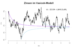
Finance:Vasicek model

Short description: Mathematical model of interest rates

A trajectory of the short rate and the corresponding yield curves at T=0 (purple) and two later points in time

In finance, the Vasicek model is a mathematical model describing the evolution of interest rates. It is a type of one-factor short-rate model as it describes interest rate movements as driven by only one source of market risk. The model can be used in the valuation of interest rate derivatives, and has also been adapted for credit markets. It was introduced in 1977 by Oldřich Vašíček, and can be also seen as a stochastic investment model.

Details

The model specifies that the instantaneous interest rate follows the stochastic differential equation:

[math]\displaystyle{ dr_t= a(b-r_t)\, dt + \sigma \, dW_t }[/math]

where W_t is a Wiener process under the risk neutral framework modelling the random market risk factor, in that it models the continuous inflow of randomness into the system. The standard deviation parameter, [math]\displaystyle{ \sigma }[/math], determines the volatility of the interest rate and in a way characterizes the amplitude of the instantaneous randomness inflow. The typical parameters [math]\displaystyle{ b, a }[/math] and [math]\displaystyle{ \sigma }[/math], together with the initial condition [math]\displaystyle{ r_0 }[/math], completely characterize the dynamics, and can be quickly characterized as follows, assuming [math]\displaystyle{ a }[/math] to be non-negative:

• [math]\displaystyle{ b }[/math]: "long term mean level". All future trajectories of [math]\displaystyle{ r }[/math] will evolve around a mean level b in the long run;
• [math]\displaystyle{ a }[/math]: "speed of reversion". [math]\displaystyle{ a }[/math] characterizes the velocity at which such trajectories will regroup around [math]\displaystyle{ b }[/math] in time;
• [math]\displaystyle{ \sigma }[/math]: "instantaneous volatility", measures instant by instant the amplitude of randomness entering the system. Higher [math]\displaystyle{ \sigma }[/math] implies more randomness

The following derived quantity is also of interest,

• [math]\displaystyle{ {\sigma^2}/(2 a) }[/math]: "long term variance". All future trajectories of [math]\displaystyle{ r }[/math] will regroup around the long term mean with such variance after a long time.

[math]\displaystyle{ a }[/math] and [math]\displaystyle{ \sigma }[/math] tend to oppose each other: increasing [math]\displaystyle{ \sigma }[/math] increases the amount of randomness entering the system, but at the same time increasing [math]\displaystyle{ a }[/math] amounts to increasing the speed at which the system will stabilize statistically around the long term mean [math]\displaystyle{ b }[/math] with a corridor of variance determined also by [math]\displaystyle{ a }[/math]. This is clear when looking at the long term variance,

[math]\displaystyle{ \frac{\sigma^2}{2 a} }[/math]

which increases with [math]\displaystyle{ \sigma }[/math] but decreases with [math]\displaystyle{ a }[/math].

This model is an Ornstein–Uhlenbeck stochastic process. Making the long term mean stochastic to another SDE is a simplified version of the cointelation SDE.

Discussion

Vasicek's model was the first one to capture mean reversion, an essential characteristic of the interest rate that sets it apart from other financial prices. Thus, as opposed to stock prices for instance, interest rates cannot rise indefinitely. This is because at very high levels they would hamper economic activity, prompting a decrease in interest rates. Similarly, interest rates do not usually decrease below 0. As a result, interest rates move in a limited range, showing a tendency to revert to a long run value.

The drift factor [math]\displaystyle{ a(b-r_t) }[/math] represents the expected instantaneous change in the interest rate at time t. The parameter b represents the long-run equilibrium value towards which the interest rate reverts. Indeed, in the absence of shocks ([math]\displaystyle{ dW_t = 0 }[/math]), the interest rate remains constant when r_t = b. The parameter a, governing the speed of adjustment, needs to be positive to ensure stability around the long term value. For example, when r_t is below b, the drift term [math]\displaystyle{ a(b-r_t) }[/math] becomes positive for positive a, generating a tendency for the interest rate to move upwards (toward equilibrium).

The main disadvantage is that, under Vasicek's model, it is theoretically possible for the interest rate to become negative, an undesirable feature under pre-crisis assumptions. This shortcoming was fixed in the Cox–Ingersoll–Ross model, exponential Vasicek model, Black–Derman–Toy model and Black–Karasinski model, among many others. The Vasicek model was further extended in the Hull–White model. The Vasicek model is also a canonical example of the affine term structure model, along with the Cox–Ingersoll–Ross model. In recent research both models were used for data partitioning and forecasting.

Asymptotic mean and variance

We solve the stochastic differential equation to obtain

[math]\displaystyle{ r_t = r_0 e^{-a t} + b\left(1- e^{-a t}\right) + \sigma e^{-a t}\int_0^t e^{a s}\,dW_s.\,\! }[/math]

Using similar techniques as applied to the Ornstein–Uhlenbeck stochastic process we get that state variable is distributed normally with mean

[math]\displaystyle{ \mathrm{E}[r_t] = r_0 e^{-a t} + b(1 - e^{-at}) }[/math]

and variance

[math]\displaystyle{ \mathrm{Var}[r_t] = \frac{\sigma^2}{2 a}(1 - e^{-2at}). }[/math]

Consequently, we have

[math]\displaystyle{ \lim_{t \to \infty} \mathrm{E}[r_t] = b }[/math]

and

[math]\displaystyle{ \lim_{t \to \infty} \mathrm{Var}[r_t] = \frac{\sigma^2}{2 a}. }[/math]

Bond pricing

Under the no-arbitrage assumption, a discount bond may be priced in the Vasicek model. The time [math]\displaystyle{ t }[/math] value of a discount bond with maturity date [math]\displaystyle{ T }[/math] is exponential affine in the interest rate:

[math]\displaystyle{ P(t,T) = e^{A(t,T) - B(t,T)r(t)} }[/math]

where

[math]\displaystyle{ B(t,T) = \frac{1 - e^{-a(T-t)}}{a} }[/math]

[math]\displaystyle{ A(t,T) = \left(b - \frac{\sigma^2}{2a^2}\right)\left[B(t,T) - (T-t)\right] - \frac{\sigma^2}{4a}B^2(t,T) }[/math]

See also

• Ornstein–Uhlenbeck process.
• Hull–White model
• Cox–Ingersoll–Ross model

References

• Hull, John C. (2003). Options, Futures and Other Derivatives. Upper Saddle River, NJ: Prentice Hall. ISBN 978-0-13-009056-0. https://archive.org/details/optionsfuturesot00hull_1. 
• Damiano Brigo, Fabio Mercurio (2001). Interest Rate Models – Theory and Practice with Smile, Inflation and Credit (2nd ed. 2006 ed.). Springer Verlag. ISBN 978-3-540-22149-4. 
• Jessica James, Nick Webber (2000). Interest Rate Modelling. Wiley. ISBN 978-0-471-97523-6. 

External links

• The Vasicek Model, Bjørn Eraker, Wisconsin School of Business
• Yield Curve Estimation and Prediction with the Vasicek Model, D. Bayazit, Middle East Technical University

References

- ↑ Vasicek, O. (1977). "An equilibrium characterization of the term structure". Journal of Financial Economics 5 (2): 177–188. doi:10.1016/0304-405X(77)90016-2.
- ↑ Mahdavi Damghani B. (2013). "The Non-Misleading Value of Inferred Correlation: An Introduction to the Cointelation Model". Wilmott Magazine 2013 (67): 50–61. doi:10.1002/wilm.10252.
- ↑ Orlando, Giuseppe; Mininni, Rosa Maria; Bufalo, Michele (July 2020). "Forecasting interest rates through Vasicek and CIR models: A partitioning approach" (in en). Journal of Forecasting 39 (4): 569–579. doi:10.1002/for.2642. ISSN 0277-6693. https://onlinelibrary.wiley.com/doi/10.1002/for.2642.