Generalization error
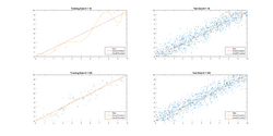
For supervised learning applications in machine learning and statistical learning theory, generalization error[1] (also known as the out-of-sample error[2] or the risk) is a measure of how accurately an algorithm is able to predict outcomes for previously unseen data. As learning algorithms are evaluated on finite samples, the evaluation of a learning algorithm may be sensitive to sampling error. As a result, measurements of prediction error on the current data may not provide much information about the algorithm's predictive ability on new, unseen data. The generalization error can be minimized by avoiding overfitting in the learning algorithm. The performance of machine learning algorithms is commonly visualized by learning curve plots that show estimates of the generalization error throughout the learning process.
Definition
In a learning problem, the goal is to develop a function that predicts output values for each input datum . The subscript indicates that the function is developed based on a data set of data points. The generalization error or expected loss or risk of a particular function over all possible values of and is the expected value of the loss function :[1]
where is the unknown joint probability distribution for and .
Without knowing the joint probability distribution , it is impossible to compute . Instead, we can compute the error on sample data, which is called empirical error (or empirical risk). Given data points, the empirical error of a candidate function is:
An algorithm is said to generalize if:
Of particular importance is the generalization error of the data-dependent function that is found by a learning algorithm based on the sample. Again, for an unknown probability distribution, cannot be computed. Instead, the aim of many problems in statistical learning theory is to bound or characterize the difference of the generalization error and the empirical error in probability:
That is, the goal is to characterize the probability that the generalization error is less than the empirical error plus some error bound (generally dependent on and ). For many types of algorithms, it has been shown that an algorithm has generalization bounds if it meets certain stability criteria. Specifically, if an algorithm is symmetric (the order of inputs does not affect the result), has bounded loss and meets two stability conditions, it will generalize. The first stability condition, leave-one-out cross-validation stability, says that to be stable, the prediction error for each data point when leave-one-out cross validation is used must converge to zero as . The second condition, expected-to-leave-one-out error stability (also known as hypothesis stability if operating in the norm) is met if the prediction on a left-out datapoint does not change when a single data point is removed from the training dataset.[3]
These conditions can be formalized as:
Leave-one-out cross-validation Stability
An algorithm has stability if for each , there exists a and such that:
and and go to zero as goes to infinity.[3]
Expected-leave-one-out error Stability
An algorithm has stability if for each there exists a and a such that:
with and going to zero for .
For leave-one-out stability in the norm, this is the same as hypothesis stability:
with going to zero as goes to infinity.[3]
Algorithms with proven stability
A number of algorithms have been proven to be stable and as a result have bounds on their generalization error. A list of these algorithms and the papers that proved stability is available here.
Relation to overfitting

The concepts of generalization error and overfitting are closely related. Overfitting occurs when the learned function becomes sensitive to the noise in the sample. As a result, the function will perform well on the training set but not perform well on other data from the joint probability distribution of and . Thus, the more overfitting occurs, the larger the generalization error.
The amount of overfitting can be tested using cross-validation methods, that split the sample into simulated training samples and testing samples. The model is then trained on a training sample and evaluated on the testing sample. The testing sample is previously unseen by the algorithm and so represents a random sample from the joint probability distribution of and . This test sample allows us to approximate the expected error and as a result approximate a particular form of the generalization error.
Many algorithms exist to prevent overfitting. The minimization algorithm can penalize more complex functions (known as Tikhonov regularization), or the hypothesis space can be constrained, either explicitly in the form of the functions or by adding constraints to the minimization function (Ivanov regularization).
The approach to finding a function that does not overfit is at odds with the goal of finding a function that is sufficiently complex to capture the particular characteristics of the data. This is known as the bias–variance tradeoff. Keeping a function simple to avoid overfitting may introduce a bias in the resulting predictions, while allowing it to be more complex leads to overfitting and a higher variance in the predictions. It is impossible to minimize both simultaneously.
References
- ↑ 1.0 1.1 Mohri, M., Rostamizadeh A., Talwakar A., (2018) Foundations of Machine learning, 2nd ed., Boston: MIT Press
- ↑ Y S. Abu-Mostafa, M.Magdon-Ismail, and H.-T. Lin (2012) Learning from Data, AMLBook Press. ISBN 978-1600490064
- ↑ 3.0 3.1 3.2 Mukherjee, S.; Niyogi, P.; Poggio, T.; Rifkin., R. M. (2006). "Learning theory: stability is sufficient for generalization and necessary and sufficient for consistency of empirical risk minimization.". Adv. Comput. Math. 25 (1–3): 161–193. doi:10.1007/s10444-004-7634-z. http://cbcl.mit.edu/publications/ps/mukherjee-ACM-06.pdf.
Further reading
- Olivier, Bousquet; Luxburg, Ulrike; Rätsch, Gunnar, eds (2004). Advanced Lectures on Machine Learning. Lecture Notes in Computer Science. 3176. pp. 169–207. doi:10.1007/b100712. ISBN 978-3-540-23122-6. https://link.springer.com/book/10.1007/b100712. Retrieved 10 December 2022.
- Bousquet, Olivier; Elisseeff, Andr´e (1 March 2002). "Stability and Generalization". The Journal of Machine Learning Research 2: 499–526. doi:10.1162/153244302760200704. https://dl.acm.org/doi/pdf/10.1162/153244302760200704. Retrieved 10 December 2022.
- Mohri, M., Rostamizadeh A., Talwakar A., (2018) Foundations of Machine learning, 2nd ed., Boston: MIT Press.
- Moody, J.E. (1992), "The Effective Number of Parameters: An Analysis of Generalization and Regularization in Nonlinear Learning Systems ", in Moody, J.E., Hanson, S.J., and Lippmann, R.P., Advances in Neural Information Processing Systems 4, 847–854.
- White, H. (1992b), Artificial Neural Networks: Approximation and Learning Theory, Blackwell.
 |

