Gene expression programming

Short description: Evolutionary algorithm

In computer programming, gene expression programming (GEP) is an evolutionary algorithm that creates computer programs or models. These computer programs are complex tree structures that learn and adapt by changing their sizes, shapes, and composition, much like a living organism. And like living organisms, the computer programs of GEP are also encoded in simple linear chromosomes of fixed length. Thus, GEP is a genotype–phenotype system, benefiting from a simple genome to keep and transmit the genetic information and a complex phenotype to explore the environment and adapt to it.

Background

Evolutionary algorithms use populations of individuals, select individuals according to fitness, and introduce genetic variation using one or more genetic operators. Their use in artificial computational systems dates back to the 1950s where they were used to solve optimization problems (e.g. Box 1957 and Friedman 1959). But it was with the introduction of evolution strategies by Rechenberg in 1965 that evolutionary algorithms gained popularity. A good overview text on evolutionary algorithms is the book "An Introduction to Genetic Algorithms" by Mitchell (1996).

Gene expression programming belongs to the family of evolutionary algorithms and is closely related to genetic algorithms and genetic programming. From genetic algorithms it inherited the linear chromosomes of fixed length; and from genetic programming it inherited the expressive parse trees of varied sizes and shapes.

In gene expression programming the linear chromosomes work as the genotype and the parse trees as the phenotype, creating a genotype/phenotype system. This genotype/phenotype system is multigenic, thus encoding multiple parse trees in each chromosome. This means that the computer programs created by GEP are composed of multiple parse trees. Because these parse trees are the result of gene expression, in GEP they are called expression trees. Masood Nekoei, et al. utilized this expression programming style in ABC optimization to conduct ABCEP as a method that outperformed other evolutionary algorithms.ABCEP

Encoding: the genotype

The genome of gene expression programming consists of a linear, symbolic string or chromosome of fixed length composed of one or more genes of equal size. These genes, despite their fixed length, code for expression trees of different sizes and shapes. An example of a chromosome with two genes, each of size 9, is the string (position zero indicates the start of each gene):

012345678012345678

L+a-baccd**cLabacd

where “L” represents the natural logarithm function and “a”, “b”, “c”, and “d” represent the variables and constants used in a problem.

Expression trees: the phenotype

As shown above, the genes of gene expression programming have all the same size. However, these fixed length strings code for expression trees of different sizes. This means that the size of the coding regions varies from gene to gene, allowing for adaptation and evolution to occur smoothly.

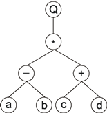
For example, the mathematical expression:

[math]\displaystyle{ \sqrt{(a-b)(c+d)} \, }[/math]

can also be represented as an expression tree:

where "Q” represents the square root function.

This kind of expression tree consists of the phenotypic expression of GEP genes, whereas the genes are linear strings encoding these complex structures. For this particular example, the linear string corresponds to:

01234567

Q*-+abcd

which is the straightforward reading of the expression tree from top to bottom and from left to right. These linear strings are called k-expressions (from Karva notation).

Going from k-expressions to expression trees is also very simple. For example, the following k-expression:

01234567890

Q*b**+baQba

is composed of two different terminals (the variables “a” and “b”), two different functions of two arguments (“*” and “+”), and a function of one argument (“Q”). Its expression gives:

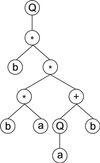
K-expressions and genes

The k-expressions of gene expression programming correspond to the region of genes that gets expressed. This means that there might be sequences in the genes that are not expressed, which is indeed true for most genes. The reason for these noncoding regions is to provide a buffer of terminals so that all k-expressions encoded in GEP genes correspond always to valid programs or expressions.

The genes of gene expression programming are therefore composed of two different domains – a head and a tail – each with different properties and functions. The head is used mainly to encode the functions and variables chosen to solve the problem at hand, whereas the tail, while also used to encode the variables, provides essentially a reservoir of terminals to ensure that all programs are error-free.

For GEP genes the length of the tail is given by the formula:

[math]\displaystyle{ t = h(n_\max-1)+1 }[/math]

where h is the head's length and n_max is maximum arity. For example, for a gene created using the set of functions F = {Q, +, −, ∗, /} and the set of terminals T = {a, b}, n_max = 2. And if we choose a head length of 15, then t = 15 (2–1) + 1 = 16, which gives a gene length g of 15 + 16 = 31. The randomly generated string below is an example of one such gene:

0123456789012345678901234567890

*b+a-aQab+//+b+babbabbbababbaaa

It encodes the expression tree:

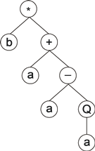
which, in this case, only uses 8 of the 31 elements that constitute the gene.

It's not hard to see that, despite their fixed length, each gene has the potential to code for expression trees of different sizes and shapes, with the simplest composed of only one node (when the first element of a gene is a terminal) and the largest composed of as many nodes as there are elements in the gene (when all the elements in the head are functions with maximum arity).

It's also not hard to see that it is trivial to implement all kinds of genetic modification (mutation, inversion, insertion, recombination, and so on) with the guarantee that all resulting offspring encode correct, error-free programs.

Multigenic chromosomes

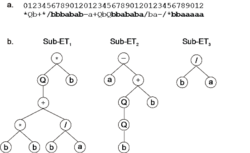
The chromosomes of gene expression programming are usually composed of more than one gene of equal length. Each gene codes for a sub-expression tree (sub-ET) or sub-program. Then the sub-ETs can interact with one another in different ways, forming a more complex program. The figure shows an example of a program composed of three sub-ETs.

Expression of GEP genes as sub-ETs. a) A three-genic chromosome with the tails shown in bold. b) The sub-ETs encoded by each gene.

In the final program the sub-ETs could be linked by addition or some other function, as there are no restrictions to the kind of linking function one might choose. Some examples of more complex linkers include taking the average, the median, the midrange, thresholding their sum to make a binomial classification, applying the sigmoid function to compute a probability, and so on. These linking functions are usually chosen a priori for each problem, but they can also be evolved elegantly and efficiently by the cellular system of gene expression programming.

Cells and code reuse

In gene expression programming, homeotic genes control the interactions of the different sub-ETs or modules of the main program. The expression of such genes results in different main programs or cells, that is, they determine which genes are expressed in each cell and how the sub-ETs of each cell interact with one another. In other words, homeotic genes determine which sub-ETs are called upon and how often in which main program or cell and what kind of connections they establish with one another.

Homeotic genes and the cellular system

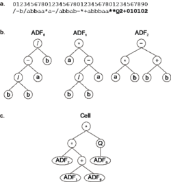
Homeotic genes have exactly the same kind of structural organization as normal genes and they are built using an identical process. They also contain a head domain and a tail domain, with the difference that the heads contain now linking functions and a special kind of terminals – genic terminals – that represent the normal genes. The expression of the normal genes results as usual in different sub-ETs, which in the cellular system are called ADFs (automatically defined functions). As for the tails, they contain only genic terminals, that is, derived features generated on the fly by the algorithm.

For example, the chromosome in the figure has three normal genes and one homeotic gene and encodes a main program that invokes three different functions a total of four times, linking them in a particular way.

Expression of a unicellular system with three ADFs. a) The chromosome composed of three conventional genes and one homeotic gene (shown in bold). b) The ADFs encoded by each conventional gene. c) The main program or cell.

From this example it is clear that the cellular system not only allows the unconstrained evolution of linking functions but also code reuse. And it shouldn't be hard to implement recursion in this system.

Multiple main programs and multicellular systems

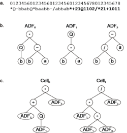
Multicellular systems are composed of more than one homeotic gene. Each homeotic gene in this system puts together a different combination of sub-expression trees or ADFs, creating multiple cells or main programs.

For example, the program shown in the figure was created using a cellular system with two cells and three normal genes.

Expression of a multicellular system with three ADFs and two main programs. a) The chromosome composed of three conventional genes and two homeotic genes (shown in bold). b) The ADFs encoded by each conventional gene. c) Two different main programs expressed in two different cells.

The applications of these multicellular systems are multiple and varied and, like the multigenic systems, they can be used both in problems with just one output and in problems with multiple outputs.

Other levels of complexity

The head/tail domain of GEP genes (both normal and homeotic) is the basic building block of all GEP algorithms. However, gene expression programming also explores other chromosomal organizations that are more complex than the head/tail structure. Essentially these complex structures consist of functional units or genes with a basic head/tail domain plus one or more extra domains. These extra domains usually encode random numerical constants that the algorithm relentlessly fine-tunes in order to find a good solution. For instance, these numerical constants may be the weights or factors in a function approximation problem (see the GEP-RNC algorithm below); they may be the weights and thresholds of a neural network (see the GEP-NN algorithm below); the numerical constants needed for the design of decision trees (see the GEP-DT algorithm below); the weights needed for polynomial induction; or the random numerical constants used to discover the parameter values in a parameter optimization task.

The basic gene expression algorithm

The fundamental steps of the basic gene expression algorithm are listed below in pseudocode:

1. Select function set;
2. Select terminal set;
3. Load dataset for fitness evaluation;
4. Create chromosomes of initial population randomly;
5. For each program in population:
   1. Express chromosome;
   2. Execute program;
   3. Evaluate fitness;
6. Verify stop condition;
7. Select programs;
8. Replicate selected programs to form the next population;
9. Modify chromosomes using genetic operators;
10. Go to step 5.

The first four steps prepare all the ingredients that are needed for the iterative loop of the algorithm (steps 5 through 10). Of these preparative steps, the crucial one is the creation of the initial population, which is created randomly using the elements of the function and terminal sets.

Populations of programs

Like all evolutionary algorithms, gene expression programming works with populations of individuals, which in this case are computer programs. Therefore, some kind of initial population must be created to get things started. Subsequent populations are descendants, via selection and genetic modification, of the initial population.

In the genotype/phenotype system of gene expression programming, it is only necessary to create the simple linear chromosomes of the individuals without worrying about the structural soundness of the programs they code for, as their expression always results in syntactically correct programs.

Fitness functions and the selection environment

Fitness functions and selection environments (called training datasets in machine learning) are the two facets of fitness and are therefore intricately connected. Indeed, the fitness of a program depends not only on the cost function used to measure its performance but also on the training data chosen to evaluate fitness

The selection environment or training data

The selection environment consists of the set of training records, which are also called fitness cases. These fitness cases could be a set of observations or measurements concerning some problem, and they form what is called the training dataset.

The quality of the training data is essential for the evolution of good solutions. A good training set should be representative of the problem at hand and also well-balanced, otherwise the algorithm might get stuck at some local optimum. In addition, it is also important to avoid using unnecessarily large datasets for training as this will slow things down unnecessarily. A good rule of thumb is to choose enough records for training to enable a good generalization in the validation data and leave the remaining records for validation and testing.

Fitness functions

Broadly speaking, there are essentially three different kinds of problems based on the kind of prediction being made:

1. Problems involving numeric (continuous) predictions;
2. Problems involving categorical or nominal predictions, both binomial and multinomial;
3. Problems involving binary or Boolean predictions.

The first type of problem goes by the name of regression; the second is known as classification, with logistic regression as a special case where, besides the crisp classifications like "Yes" or "No", a probability is also attached to each outcome; and the last one is related to Boolean algebra and logic synthesis.

Fitness functions for regression

In regression, the response or dependent variable is numeric (usually continuous) and therefore the output of a regression model is also continuous. So it's quite straightforward to evaluate the fitness of the evolving models by comparing the output of the model to the value of the response in the training data.

There are several basic fitness functions for evaluating model performance, with the most common being based on the error or residual between the model output and the actual value. Such functions include the mean squared error, root mean squared error, mean absolute error, relative squared error, root relative squared error, relative absolute error, and others.

All these standard measures offer a fine granularity or smoothness to the solution space and therefore work very well for most applications. But some problems might require a coarser evolution, such as determining if a prediction is within a certain interval, for instance less than 10% of the actual value. However, even if one is only interested in counting the hits (that is, a prediction that is within the chosen interval), making populations of models evolve based on just the number of hits each program scores is usually not very efficient due to the coarse granularity of the fitness landscape. Thus the solution usually involves combining these coarse measures with some kind of smooth function such as the standard error measures listed above.

Fitness functions based on the correlation coefficient and R-square are also very smooth. For regression problems, these functions work best by combining them with other measures because, by themselves, they only tend to measure correlation, not caring for the range of values of the model output. So by combining them with functions that work at approximating the range of the target values, they form very efficient fitness functions for finding models with good correlation and good fit between predicted and actual values.

Fitness functions for classification and logistic regression

The design of fitness functions for classification and logistic regression takes advantage of three different characteristics of classification models. The most obvious is just counting the hits, that is, if a record is classified correctly it is counted as a hit. This fitness function is very simple and works well for simple problems, but for more complex problems or datasets highly unbalanced it gives poor results.

One way to improve this type of hits-based fitness function consists of expanding the notion of correct and incorrect classifications. In a binary classification task, correct classifications can be 00 or 11. The "00" representation means that a negative case (represented by "0”) was correctly classified, whereas the "11" means that a positive case (represented by "1”) was correctly classified. Classifications of the type "00" are called true negatives (TN) and "11" true positives (TP).

There are also two types of incorrect classifications and they are represented by 01 and 10. They are called false positives (FP) when the actual value is 0 and the model predicts a 1; and false negatives (FN) when the target is 1 and the model predicts a 0. The counts of TP, TN, FP, and FN are usually kept on a table known as the confusion matrix.

Confusion matrix for a binomial classification task.

		Predicted class
		Yes	No
rowspan="2"	Yes	TP	FN
No	FP	TN

So by counting the TP, TN, FP, and FN and further assigning different weights to these four types of classifications, it is possible to create smoother and therefore more efficient fitness functions. Some popular fitness functions based on the confusion matrix include sensitivity/specificity, recall/precision, F-measure, Jaccard similarity, Matthews correlation coefficient, and cost/gain matrix which combines the costs and gains assigned to the 4 different types of classifications.

These functions based on the confusion matrix are quite sophisticated and are adequate to solve most problems efficiently. But there is another dimension to classification models which is key to exploring more efficiently the solution space and therefore results in the discovery of better classifiers. This new dimension involves exploring the structure of the model itself, which includes not only the domain and range, but also the distribution of the model output and the classifier margin.

By exploring this other dimension of classification models and then combining the information about the model with the confusion matrix, it is possible to design very sophisticated fitness functions that allow the smooth exploration of the solution space. For instance, one can combine some measure based on the confusion matrix with the mean squared error evaluated between the raw model outputs and the actual values. Or combine the F-measure with the R-square evaluated for the raw model output and the target; or the cost/gain matrix with the correlation coefficient, and so on. More exotic fitness functions that explore model granularity include the area under the ROC curve and rank measure.

Also related to this new dimension of classification models, is the idea of assigning probabilities to the model output, which is what is done in logistic regression. Then it is also possible to use these probabilities and evaluate the mean squared error (or some other similar measure) between the probabilities and the actual values, then combine this with the confusion matrix to create very efficient fitness functions for logistic regression. Popular examples of fitness functions based on the probabilities include maximum likelihood estimation and hinge loss.

Fitness functions for Boolean problems

In logic there is no model structure (as defined above for classification and logistic regression) to explore: the domain and range of logical functions comprises only 0's and 1's or false and true. So, the fitness functions available for Boolean algebra can only be based on the hits or on the confusion matrix as explained in the section above.

Selection and elitism

Roulette-wheel selection is perhaps the most popular selection scheme used in evolutionary computation. It involves mapping the fitness of each program to a slice of the roulette wheel proportional to its fitness. Then the roulette is spun as many times as there are programs in the population in order to keep the population size constant. So, with roulette-wheel selection programs are selected both according to fitness and the luck of the draw, which means that some times the best traits might be lost. However, by combining roulette-wheel selection with the cloning of the best program of each generation, one guarantees that at least the very best traits are not lost. This technique of cloning the best-of-generation program is known as simple elitism and is used by most stochastic selection schemes.

Reproduction with modification

The reproduction of programs involves first the selection and then the reproduction of their genomes. Genome modification is not required for reproduction, but without it adaptation and evolution won't take place.

Replication and selection

The selection operator selects the programs for the replication operator to copy. Depending on the selection scheme, the number of copies one program originates may vary, with some programs getting copied more than once while others are copied just once or not at all. In addition, selection is usually set up so that the population size remains constant from one generation to another.

The replication of genomes in nature is very complex and it took scientists a long time to discover the DNA double helix and propose a mechanism for its replication. But the replication of strings is trivial in artificial evolutionary systems, where only an instruction to copy strings is required to pass all the information in the genome from generation to generation.

The replication of the selected programs is a fundamental piece of all artificial evolutionary systems, but for evolution to occur it needs to be implemented not with the usual precision of a copy instruction, but rather with a few errors thrown in. Indeed, genetic diversity is created with genetic operators such as mutation, recombination, transposition, inversion, and many others.

Mutation

In gene expression programming mutation is the most important genetic operator. It changes genomes by changing an element by another. The accumulation of many small changes over time can create great diversity.

In gene expression programming mutation is totally unconstrained, which means that in each gene domain any domain symbol can be replaced by another. For example, in the heads of genes any function can be replaced by a terminal or another function, regardless of the number of arguments in this new function; and a terminal can be replaced by a function or another terminal.

Recombination

Recombination usually involves two parent chromosomes to create two new chromosomes by combining different parts from the parent chromosomes. And as long as the parent chromosomes are aligned and the exchanged fragments are homologous (that is, occupy the same position in the chromosome), the new chromosomes created by recombination will always encode syntactically correct programs.

Different kinds of crossover are easily implemented either by changing the number of parents involved (there's no reason for choosing only two); the number of split points; or the way one chooses to exchange the fragments, for example, either randomly or in some orderly fashion. For example, gene recombination, which is a special case of recombination, can be done by exchanging homologous genes (genes that occupy the same position in the chromosome) or by exchanging genes chosen at random from any position in the chromosome.

Transposition

Transposition involves the introduction of an insertion sequence somewhere in a chromosome. In gene expression programming insertion sequences might appear anywhere in the chromosome, but they are only inserted in the heads of genes. This method guarantees that even insertion sequences from the tails result in error-free programs.

For transposition to work properly, it must preserve chromosome length and gene structure. So, in gene expression programming transposition can be implemented using two different methods: the first creates a shift at the insertion site, followed by a deletion at the end of the head; the second overwrites the local sequence at the target site and therefore is easier to implement. Both methods can be implemented to operate between chromosomes or within a chromosome or even within a single gene.

Inversion

Inversion is an interesting operator, especially powerful for combinatorial optimization. It consists of inverting a small sequence within a chromosome.

In gene expression programming it can be easily implemented in all gene domains and, in all cases, the offspring produced is always syntactically correct. For any gene domain, a sequence (ranging from at least two elements to as big as the domain itself) is chosen at random within that domain and then inverted.

Other genetic operators

Several other genetic operators exist and in gene expression programming, with its different genes and gene domains, the possibilities are endless. For example, genetic operators such as one-point recombination, two-point recombination, gene recombination, uniform recombination, gene transposition, root transposition, domain-specific mutation, domain-specific inversion, domain-specific transposition, and so on, are easily implemented and widely used.

The GEP-RNC algorithm

Numerical constants are essential elements of mathematical and statistical models and therefore it is important to allow their integration in the models designed by evolutionary algorithms.

Gene expression programming solves this problem very elegantly through the use of an extra gene domain – the Dc – for handling random numerical constants (RNC). By combining this domain with a special terminal placeholder for the RNCs, a richly expressive system can be created.

Structurally, the Dc comes after the tail, has a length equal to the size of the tail t, and is composed of the symbols used to represent the RNCs.

For example, below is shown a simple chromosome composed of only one gene a head size of 7 (the Dc stretches over positions 15–22):

01234567890123456789012

+?*+?**aaa??aaa68083295

where the terminal "?” represents the placeholder for the RNCs. This kind of chromosome is expressed exactly as shown above, giving:

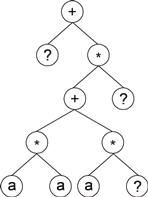
Then the ?'s in the expression tree are replaced from left to right and from top to bottom by the symbols (for simplicity represented by numerals) in the Dc, giving:

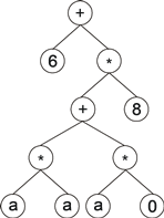
The values corresponding to these symbols are kept in an array. (For simplicity, the number represented by the numeral indicates the order in the array.) For instance, for the following 10 element array of RNCs:

C = {0.611, 1.184, 2.449, 2.98, 0.496, 2.286, 0.93, 2.305, 2.737, 0.755}

the expression tree above gives:

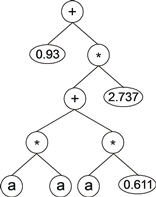
This elegant structure for handling random numerical constants is at the heart of different GEP systems, such as GEP neural networks and GEP decision trees.

Like the basic gene expression algorithm, the GEP-RNC algorithm is also multigenic and its chromosomes are decoded as usual by expressing one gene after another and then linking them all together by the same kind of linking process.

The genetic operators used in the GEP-RNC system are an extension to the genetic operators of the basic GEP algorithm (see above), and they all can be straightforwardly implemented in these new chromosomes. On the other hand, the basic operators of mutation, inversion, transposition, and recombination are also used in the GEP-RNC algorithm. Furthermore, special Dc-specific operators such as mutation, inversion, and transposition, are also used to aid in a more efficient circulation of the RNCs among individual programs. In addition, there is also a special mutation operator that allows the permanent introduction of variation in the set of RNCs. The initial set of RNCs is randomly created at the beginning of a run, which means that, for each gene in the initial population, a specified number of numerical constants, chosen from a certain range, are randomly generated. Then their circulation and mutation is enabled by the genetic operators.

Neural networks

An artificial neural network (ANN or NN) is a computational device that consists of many simple connected units or neurons. The connections between the units are usually weighted by real-valued weights. These weights are the primary means of learning in neural networks and a learning algorithm is usually used to adjust them.

Structurally, a neural network has three different classes of units: input units, hidden units, and output units. An activation pattern is presented at the input units and then spreads in a forward direction from the input units through one or more layers of hidden units to the output units. The activation coming into one unit from other unit is multiplied by the weights on the links over which it spreads. All incoming activation is then added together and the unit becomes activated only if the incoming result is above the unit's threshold.

In summary, the basic components of a neural network are the units, the connections between the units, the weights, and the thresholds. So, in order to fully simulate an artificial neural network one must somehow encode these components in a linear chromosome and then be able to express them in a meaningful way.

In GEP neural networks (GEP-NN or GEP nets), the network architecture is encoded in the usual structure of a head/tail domain. The head contains special functions/neurons that activate the hidden and output units (in the GEP context, all these units are more appropriately called functional units) and terminals that represent the input units. The tail, as usual, contains only terminals/input units.

Besides the head and the tail, these neural network genes contain two additional domains, Dw and Dt, for encoding the weights and thresholds of the neural network. Structurally, the Dw comes after the tail and its length d_w depends on the head size h and maximum arity n_max and is evaluated by the formula:

[math]\displaystyle{ d_{w} = hn_\max }[/math]

The Dt comes after Dw and has a length d_t equal to t. Both domains are composed of symbols representing the weights and thresholds of the neural network.

For each NN-gene, the weights and thresholds are created at the beginning of each run, but their circulation and adaptation are guaranteed by the usual genetic operators of mutation, transposition, inversion, and recombination. In addition, special operators are also used to allow a constant flow of genetic variation in the set of weights and thresholds.

For example, below is shown a neural network with two input units (i₁ and i₂), two hidden units (h₁ and h₂), and one output unit (o₁). It has a total of six connections with six corresponding weights represented by the numerals 1–6 (for simplicity, the thresholds are all equal to 1 and are omitted):

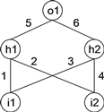
This representation is the canonical neural network representation, but neural networks can also be represented by a tree, which, in this case, corresponds to:

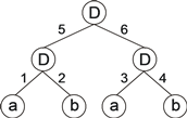
where "a” and "b” represent the two inputs i₁ and i₂ and "D” represents a function with connectivity two. This function adds all its weighted arguments and then thresholds this activation in order to determine the forwarded output. This output (zero or one in this simple case) depends on the threshold of each unit, that is, if the total incoming activation is equal to or greater than the threshold, then the output is one, zero otherwise.

The above NN-tree can be linearized as follows:

0123456789012

DDDabab654321

where the structure in positions 7–12 (Dw) encodes the weights. The values of each weight are kept in an array and retrieved as necessary for expression.

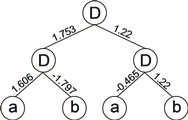
As a more concrete example, below is shown a neural net gene for the exclusive-or problem. It has a head size of 3 and Dw size of 6:

0123456789012

DDDabab393257

Its expression results in the following neural network:

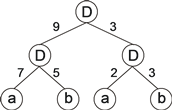
which, for the set of weights:

W = {−1.978, 0.514, −0.465, 1.22, −1.686, −1.797, 0.197, 1.606, 0, 1.753}

it gives:

which is a perfect solution to the exclusive-or function.

Besides simple Boolean functions with binary inputs and binary outputs, the GEP-nets algorithm can handle all kinds of functions or neurons (linear neuron, tanh neuron, atan neuron, logistic neuron, limit neuron, radial basis and triangular basis neurons, all kinds of step neurons, and so on). Also interesting is that the GEP-nets algorithm can use all these neurons together and let evolution decide which ones work best to solve the problem at hand. So, GEP-nets can be used not only in Boolean problems but also in logistic regression, classification, and regression. In all cases, GEP-nets can be implemented not only with multigenic systems but also cellular systems, both unicellular and multicellular. Furthermore, multinomial classification problems can also be tackled in one go by GEP-nets both with multigenic systems and multicellular systems.

Decision trees

Decision trees (DT) are classification models where a series of questions and answers are mapped using nodes and directed edges.

Decision trees have three types of nodes: a root node, internal nodes, and leaf or terminal nodes. The root node and all internal nodes represent test conditions for different attributes or variables in a dataset. Leaf nodes specify the class label for all different paths in the tree.

Most decision tree induction algorithms involve selecting an attribute for the root node and then make the same kind of informed decision about all the nodes in a tree.

Decision trees can also be created by gene expression programming, with the advantage that all the decisions concerning the growth of the tree are made by the algorithm itself without any kind of human input.

There are basically two different types of DT algorithms: one for inducing decision trees with only nominal attributes and another for inducing decision trees with both numeric and nominal attributes. This aspect of decision tree induction also carries to gene expression programming and there are two GEP algorithms for decision tree induction: the evolvable decision trees (EDT) algorithm for dealing exclusively with nominal attributes and the EDT-RNC (EDT with random numerical constants) for handling both nominal and numeric attributes.

In the decision trees induced by gene expression programming, the attributes behave as function nodes in the basic gene expression algorithm, whereas the class labels behave as terminals. This means that attribute nodes have also associated with them a specific arity or number of branches that will determine their growth and, ultimately, the growth of the tree. Class labels behave like terminals, which means that for a k-class classification task, a terminal set with k terminals is used, representing the k different classes.

The rules for encoding a decision tree in a linear genome are very similar to the rules used to encode mathematical expressions (see above). So, for decision tree induction the genes also have a head and a tail, with the head containing attributes and terminals and the tail containing only terminals. This again ensures that all decision trees designed by GEP are always valid programs. Furthermore, the size of the tail t is also dictated by the head size h and the number of branches of the attribute with more branches n_max and is evaluated by the equation:

[math]\displaystyle{ t = h(n_\max-1)+1 \, }[/math]

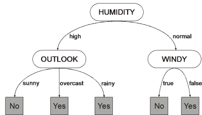
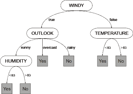
For example, consider the decision tree below to decide whether to play outside:

It can be linearly encoded as:

01234567

HOWbaaba

where “H” represents the attribute Humidity, “O” the attribute Outlook, “W” represents Windy, and “a” and “b” the class labels "Yes" and "No" respectively. Note that the edges connecting the nodes are properties of the data, specifying the type and number of branches of each attribute, and therefore don't have to be encoded.

The process of decision tree induction with gene expression programming starts, as usual, with an initial population of randomly created chromosomes. Then the chromosomes are expressed as decision trees and their fitness evaluated against a training dataset. According to fitness they are then selected to reproduce with modification. The genetic operators are exactly the same that are used in a conventional unigenic system, for example, mutation, inversion, transposition, and recombination.

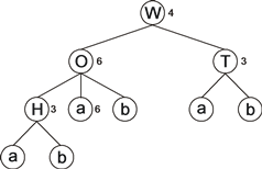
Decision trees with both nominal and numeric attributes are also easily induced with gene expression programming using the framework described above for dealing with random numerical constants. The chromosomal architecture includes an extra domain for encoding random numerical constants, which are used as thresholds for splitting the data at each branching node. For example, the gene below with a head size of 5 (the Dc starts at position 16):

012345678901234567890

WOTHabababbbabba46336

encodes the decision tree shown below:

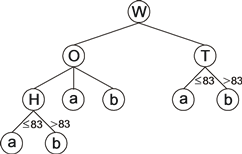
In this system, every node in the head, irrespective of its type (numeric attribute, nominal attribute, or terminal), has associated with it a random numerical constant, which for simplicity in the example above is represented by a numeral 0–9. These random numerical constants are encoded in the Dc domain and their expression follows a very simple scheme: from top to bottom and from left to right, the elements in Dc are assigned one-by-one to the elements in the decision tree. So, for the following array of RNCs:

C = {62, 51, 68, 83, 86, 41, 43, 44, 9, 67}

the decision tree above results in:

which can also be represented more colorfully as a conventional decision tree:

Criticism

GEP has been criticized for not being a major improvement over other genetic programming techniques. In many experiments, it did not perform better than existing methods.

Software

Commercial applications

GeneXproTools

GeneXproTools is a predictive analytics suite developed by Gepsoft. GeneXproTools modeling frameworks include logistic regression, classification, regression, time series prediction, and logic synthesis. GeneXproTools implements the basic gene expression algorithm and the GEP-RNC algorithm, both used in all the modeling frameworks of GeneXproTools.

Open-source libraries

GEP4J – GEP for Java Project

Created by Jason Thomas, GEP4J is an open-source implementation of gene expression programming in Java. It implements different GEP algorithms, including evolving decision trees (with nominal, numeric, or mixed attributes) and automatically defined functions. GEP4J is hosted at Google Code.

PyGEP – Gene Expression Programming for Python

Created by Ryan O'Neil with the goal to create a simple library suitable for the academic study of gene expression programming in Python, aiming for ease of use and rapid implementation. It implements standard multigenic chromosomes and the genetic operators mutation, crossover, and transposition. PyGEP is hosted at Google Code.

jGEP – Java GEP toolkit

Created by Matthew Sottile to rapidly build Java prototype codes that use GEP, which can then be written in a language such as C or Fortran for real speed. jGEP is hosted at SourceForge.

Further reading

• Ferreira, C. (2006). Gene Expression Programming: Mathematical Modeling by an Artificial Intelligence. Springer-Verlag. ISBN 3-540-32796-7. 
• Ferreira, C. (2002). Gene Expression Programming: Mathematical Modeling by an Artificial Intelligence. Portugal: Angra do Heroismo. ISBN 972-95890-5-4. http://www.gene-expression-programming.com/GepBook/Introduction.htm. 

See also

• Symbolic Regression
• Artificial intelligence
• Decision trees
• Evolutionary algorithms
• Genetic algorithms
• Genetic programming
• Grammatical evolution
• Linear genetic programming
• GeneXproTools
• Machine learning
• Multi expression programming
• Neural networks

External links

• GEP home page, maintained by the inventor of gene expression programming.
• GeneXproTools, commercial GEP software.

References

- ↑ Box, G. E. P., 1957. Evolutionary operation: A method for increasing industrial productivity. Applied Statistics, 6, 81–101.
- ↑ Friedman, G. J., 1959. Digital simulation of an evolutionary process. General Systems Yearbook, 4, 171–184.
- ↑ Rechenberg, Ingo (1973). Evolutionsstrategie. Stuttgart: Holzmann-Froboog. ISBN 3-7728-0373-3.
- ↑ Mitchell, Melanie (1996). 'An Introduction to Genetic Algorithms. Cambridge, MA: MIT Press. https://archive.org/details/introductiontoge00mitc.
- ↑ Ferreira, C. (2001). "Gene Expression Programming: A New Adaptive Algorithm for Solving Problems". Complex Systems, Vol. 13, issue 2: 87–129. http://www.gene-expression-programming.com/webpapers/GEP.pdf.