Root mean square
In mathematics, the root mean square (abbrev. RMS, RMS or rms) of a set of values is the square root of the set's mean square.[1] Given a set , its RMS is denoted as either or . The RMS is also known as the quadratic mean (denoted ),[2][3] a special case of the generalized mean. The RMS of a continuous function is denoted and can be defined in terms of an integral of the square of the function. In estimation theory, the root-mean-square deviation of an estimator measures how far the estimator strays from the data.
Definition
The RMS value of a set of values (or a continuous-time waveform) is the square root of the arithmetic mean of the squares of the values, or the square of the function that defines the continuous waveform.
In the case of a set of n values , the RMS is
The corresponding formula for a continuous function (or waveform) f(t) defined over the interval is
and the RMS for a function over all time is
The RMS over all time of a periodic function is equal to the RMS of one period of the function. The RMS value of a continuous function or signal can be approximated by taking the RMS of a sample consisting of equally spaced observations. Additionally, the RMS value of various waveforms can also be determined without calculus, as shown by Cartwright.[4]
In the case of the RMS statistic of a random process, the expected value is used instead of the mean.
In common waveforms


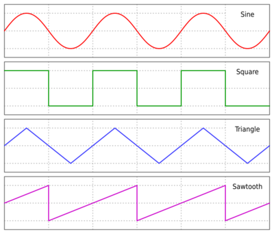
If the waveform is a pure sine wave, the relationships between amplitudes (peak-to-peak, peak) and RMS are fixed and known, as they are for any continuous periodic wave. However, this is not true for an arbitrary waveform, which may not be periodic or continuous. For a zero-mean sine wave, the relationship between RMS and peak-to-peak amplitude is:
- Peak-to-peak
For other waveforms, the relationships are not the same as they are for sine waves. For example, for either a triangular or sawtooth wave:
- Peak-to-peak
| Waveform | Variables and operators | RMS |
|---|---|---|
| DC | ||
| Sine wave | ||
| Square wave | ||
| DC-shifted square wave | ||
| Modified sine wave | ||
| Triangle wave | ||
| Sawtooth wave | ||
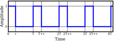
| Pulse wave | ||
| Phase-to-phase sine wave | ||
where:
| ||
In waveform combinations
Waveforms made by summing known simple waveforms have an RMS value that is the root of the sum of squares of the component RMS values, if the component waveforms are orthogonal (that is, if the average of the product of one simple waveform with another is zero for all pairs other than a waveform times itself).[5]
Alternatively, for waveforms that are perfectly positively correlated, or "in phase" with each other, their RMS values sum directly.
Uses
In electrical engineering
Current
The RMS of an alternating electric current equals the value of constant direct current that would dissipate the same power in a resistive load.[1]
Voltage
A special case of RMS of waveform combinations is:[6]
where refers to the direct current (or average) component of the signal, and is the alternating current component of the signal.
Average electrical power
Electrical engineers often need to know the power, P, dissipated by an electrical resistance, R. It is easy to do the calculation when there is a constant current, I, through the resistance. For a load of R ohms, power is given by:
However, if the current is a time-varying function, I(t), this formula must be extended to reflect the fact that the current (and thus the instantaneous power) is varying over time. If the function is periodic (such as household AC power), it is still meaningful to discuss the average power dissipated over time, which is calculated by taking the average power dissipation:
So, the RMS value, IRMS, of the function I(t) is the constant current that yields the same power dissipation as the time-averaged power dissipation of the current I(t).
Average power can also be found using the same method that in the case of a time-varying voltage, V(t), with RMS value VRMS,
This equation can be used for any periodic waveform, such as a sinusoidal or sawtooth waveform, allowing us to calculate the mean power delivered into a specified load.
By taking the square root of both these equations and multiplying them together, the power is found to be:
Both derivations depend on voltage and current being proportional (that is, the load, R, is purely resistive). Reactive loads (that is, loads capable of not just dissipating energy but also storing it) are discussed under the topic of AC power.
In the common case of alternating current when I(t) is a sinusoidal current, as is approximately true for mains power, the RMS value is easy to calculate from the continuous case equation above. If Ip is defined to be the peak current, then:
where t is time and ω is the angular frequency (ω = 2π/T, where T is the period of the wave).
Since Ip is a positive constant and was to be squared within the integral:
Using a trigonometric identity to eliminate squaring of trig function:
but since the interval is a whole number of complete cycles (per definition of RMS), the sine terms will cancel out, leaving:
A similar analysis leads to the analogous equation for sinusoidal voltage:
where IP represents the peak current and VP represents the peak voltage.
Because of their usefulness in carrying out power calculations, listed voltages for power outlets (for example, 120 V in the US, or 230 V in Europe) are almost always quoted in RMS values, and not peak values. Peak values can be calculated from RMS values from the above formula, which implies VP = VRMS × √2, assuming the source is a pure sine wave. Thus the peak value of the mains voltage in the USA is about 120 × √2, or about 170 volts. The peak-to-peak voltage, being double this, is about 340 volts. A similar calculation indicates that the peak mains voltage in Europe is about 325 volts, and the peak-to-peak mains voltage, about 650 volts.
RMS quantities such as electric current are usually calculated over one cycle. However, for some purposes the RMS current over a longer period is required when calculating transmission power losses. The same principle applies, and (for example) a current of 10 amps used for 12 hours each 24-hour day represents an average current of 5 amps, but an RMS current of 7.07 amps, in the long term.
The term RMS power is sometimes erroneously used (e.g., in the audio industry) as a synonym for mean power or average power (it is proportional to the square of the RMS voltage or RMS current in a resistive load). For a discussion of audio power measurements and their shortcomings, see Audio power.
Speed
In the physics of gas molecules, the root-mean-square speed is defined as the square root of the average squared-speed. The RMS speed of an ideal gas is calculated using the following equation:
where R represents the gas constant, 8.314 J/(mol·K), T is the temperature of the gas in kelvins, and M is the molar mass of the gas in kilograms per mole. In physics, speed is defined as the scalar magnitude of velocity. For a stationary gas, the average speed of its molecules can be in the order of thousands of km/h, even though the average velocity of its molecules is zero.
Error
When two data sets — one set from theoretical prediction and the other from actual measurement of some physical variable, for instance — are compared, the RMS of the pairwise differences of the two data sets can serve as a measure of how far on average the error is from 0. The mean of the absolute values of the pairwise differences could be a useful measure of the variability of the differences. However, the RMS of the differences is usually the preferred measure, probably due to mathematical convention and compatibility with other formulae.
Audio Engineering
RMS is used in audio engineering to measure signal volume, particularly in the case of audio processing. The alternative volume measurement is peak volume, in analog as the signal Vpp, or in digital as the -dB peak below clipping given the encoding format. Signal RMS in this context is often used as the comparator signal for compression, which produces a "smoothing" effect in compression by responding more slowly to sharp transients like those on drums.[7] RMS is also used as a mastering metric to compare against other time average units such as LUFs.[8]
In frequency domain
The RMS can be computed in the frequency domain, using Parseval's theorem. For a sampled signal , where is the sampling period,
where and N is the sample size, that is, the number of observations in the sample and DFT coefficients.
In this case, the RMS computed in the time domain is the same as in the frequency domain:
Relationship to other statistics
Template:QM AM GM HM inequality visual proof.svg The standard deviation of a population or a waveform is the RMS deviation of from its arithmetic mean . They are related to the RMS value of by [9]
- .
From this it is clear that the RMS value is always greater than or equal to the average, in that the RMS includes the squared deviation (error) as well.
Physical scientists often use the term root mean square as a synonym for standard deviation when it can be assumed the input signal has zero mean, that is, referring to the square root of the mean squared deviation of a signal from a given baseline or fit.[10][11] This is useful for electrical engineers in calculating the "AC only" RMS of a signal. Standard deviation being the RMS of a signal's variation about the mean, rather than about 0, the DC component is removed (that is, RMS(signal) = stdev(signal) if the mean signal is 0).
See also
- Average rectified value (ARV)
- Central moment
- Geometric mean
- Glossary of mathematical symbols
- L2 norm
- Least squares
- Mean squared displacement
- Pythagorean addition
- True RMS converter
Notes
References
- ↑ 1.0 1.1 "Root-mean-square value". A Dictionary of Physics (6 ed.). Oxford University Press. 2009. ISBN 9780199233991. https://www.oxfordreference.com/view/10.1093/acref/9780199233991.001.0001/acref-9780199233991-e-2676.
- ↑ Thompson, Sylvanus P. (1965). Calculus Made Easy. Macmillan International Higher Education. p. 185. ISBN 9781349004874. https://books.google.com/books?id=6VJdDwAAQBAJ&pg=PA185. Retrieved 5 July 2020.
- ↑ Jones, Alan R. (2018). Probability, Statistics and Other Frightening Stuff. Routledge. p. 48. ISBN 9781351661386. https://books.google.com/books?id=OvtsDwAAQBAJ&pg=PA48. Retrieved 5 July 2020.
- ↑ Cartwright, Kenneth V (Fall 2007). "Determining the Effective or RMS Voltage of Various Waveforms without Calculus". Technology Interface 8 (1): 20 pages. http://tiij.org/issues/issues/fall2007/30_Cartwright/Cartwright-Waveforms.pdf.
- ↑ Nastase, Adrian S.. "How to Derive the RMS Value of Pulse and Square Waveforms". https://masteringelectronicsdesign.com/how-to-derive-the-rms-value-of-pulse-and-square-waveforms/.
- ↑ "Make Better AC RMS Measurements with your Digital Multimeter". https://literature.cdn.keysight.com/litweb/pdf/5988-6916EN.pdf.
- ↑ Lessons, Alex-Mixing (2019-09-23). "Peak vs RMS compression: The difference between Peak and RMS" (in en-GB). https://www.mixinglessons.com/peak-vs-rms-compression/.
- ↑ Luthar, Margaret (June 12, 2024). "RMS levels defined: how to get consistent loudness levels in mastering". https://www.izotope.com/en/learn/rms-levels.html?srsltid=AfmBOooGSAJqXnQOsjQbXSHrtq3_gZaQ5ssxT-bKCbhxuT0HKR43nw9H.
- ↑ Chris C. Bissell; David A. Chapman (1992). Digital signal transmission (2nd ed.). Cambridge University Press. p. 64. ISBN 978-0-521-42557-5.
- ↑ Weisstein, Eric W.. "Root-Mean-Square". MathWorld. https://mathworld.wolfram.com/Root-Mean-Square.html.
- ↑ "ROOT, TH1:GetRMS". http://root.cern.ch/root/html/TH1.html#TH1:GetRMS.
External links
it:Valore efficace
 |
