Tensorsketch

Short description: Algorithm for reducing the dimension of tensors

In statistics, machine learning and algorithms, a tensor sketch is a type of dimensionality reduction that is particularly efficient when applied to vectors that have tensor structure. Such a sketch can be used to speed up explicit kernel methods, bilinear pooling in neural networks and is a cornerstone in many numerical linear algebra algorithms.

Mathematical definition

Mathematically, a dimensionality reduction is a matrix [math]\displaystyle{ M\in\mathbb R^{k,d} }[/math], where [math]\displaystyle{ k\lt d }[/math], such that for any vector [math]\displaystyle{ x\in\mathbb R^d }[/math] it holds that

[math]\displaystyle{ |\|Mx\|_2 - \|x\|_2| \lt \varepsilon\|x\|_2 }[/math]

with high probability. In other words [math]\displaystyle{ M }[/math] preserves the norm of vectors up to a small error.

A Tensor sketch has the extra property that if [math]\displaystyle{ x = y \otimes z }[/math] for some vectors [math]\displaystyle{ y\in\mathbb R^{d_1}, z\in\mathbb R^{d_2} }[/math] such that [math]\displaystyle{ d_1d_2=d }[/math], the transformation [math]\displaystyle{ M(y\otimes z) }[/math] can be computed extra efficiently.

Typically [math]\displaystyle{ M(y\otimes z) = M' y \circ M' z }[/math], where [math]\displaystyle{ \circ }[/math] is the (Hadamard) elementwise product. Since each of [math]\displaystyle{ M' y }[/math] and [math]\displaystyle{ M' z }[/math] can be computed in time respectively [math]\displaystyle{ kd_1 }[/math] and [math]\displaystyle{ kd_2 }[/math], the computation is much faster than the full [math]\displaystyle{ Mx }[/math] which would take time [math]\displaystyle{ kd=kd_1d_2 }[/math].

For higher-order tensors, such as [math]\displaystyle{ x = y\otimes z\otimes t }[/math] the savings are even more impressive.

History

The term tensor sketch was coined in 2013 describing a technique by Rasmus Pagh from the same year. Originally it was understood using the Fast Fourier Transform to do fast convolution of Count Sketches. Later research works generalized it to a much larger class of dimensionality reductions via Tensor random embeddings.

Tensor random embeddings were introduced in 2010 in a paper on differential privacy and were first analyzed by Rudelson et al. in 2012 in the context of sparse recovery.

Avron et al. were the first to study the subspace embedding properties of tensor sketches, particularly focused on applications to polynomial kernels. In this context, the sketch is required not only to preserve the norm of each individual vector with a certain probability but to preserve the norm of all vectors in each individual linear subspace. This is a much stronger property, and it requires larger sketch sizes, but it allows the kernel methods to be used very broadly as explored in the book by David Woodruff.

Tensor random projections

The face-splitting product is defined as the tensor products of the rows. More directly, let [math]\displaystyle{ \mathbf{C}\in\mathbb R^{3\times 3} }[/math] and [math]\displaystyle{ \mathbf{D}\in\mathbb R^{3\times 3} }[/math] be two matrices. Then the Face-splitting product [math]\displaystyle{ \mathbf{C}\bullet \mathbf{D} }[/math] is

[math]\displaystyle{ \mathbf{C} \bull \mathbf{D} = \left[ \begin{array} { c } \mathbf{C}_1 \otimes \mathbf{D}_1\\\hline \mathbf{C}_2 \otimes \mathbf{D}_2\\\hline \mathbf{C}_3 \otimes \mathbf{D}_3\\ \end{array} \right] = \left[ \begin{array} { c c c c c c c c c } \mathbf{C}_{1,1}\mathbf{D}_{1,1} & \mathbf{C}_{1,1}\mathbf{D}_{1,2} & \mathbf{C}_{1,1}\mathbf{D}_{1,3} & \mathbf{C}_{1,2}\mathbf{D}_{1,1} & \mathbf{C}_{1,2}\mathbf{D}_{1,2} & \mathbf{C}_{1,2}\mathbf{D}_{1,3} & \mathbf{C}_{1,3}\mathbf{D}_{1,1} & \mathbf{C}_{1,3}\mathbf{D}_{1,2} & \mathbf{C}_{1,3}\mathbf{D}_{1,3} \\\hline \mathbf{C}_{2,1}\mathbf{D}_{2,1} & \mathbf{C}_{2,1}\mathbf{D}_{2,2} & \mathbf{C}_{2,1}\mathbf{D}_{2,3} & \mathbf{C}_{2,2}\mathbf{D}_{2,1} & \mathbf{C}_{2,2}\mathbf{D}_{2,2} & \mathbf{C}_{2,2}\mathbf{D}_{2,3} & \mathbf{C}_{2,3}\mathbf{D}_{2,1} & \mathbf{C}_{2,3}\mathbf{D}_{2,2} & \mathbf{C}_{2,3}\mathbf{D}_{2,3} \\\hline \mathbf{C}_{3,1}\mathbf{D}_{3,1} & \mathbf{C}_{3,1}\mathbf{D}_{3,2} & \mathbf{C}_{3,1}\mathbf{D}_{3,3} & \mathbf{C}_{3,2}\mathbf{D}_{3,1} & \mathbf{C}_{3,2}\mathbf{D}_{3,2} & \mathbf{C}_{3,2}\mathbf{D}_{3,3} & \mathbf{C}_{3,3}\mathbf{D}_{3,1} & \mathbf{C}_{3,3}\mathbf{D}_{3,2} & \mathbf{C}_{3,3}\mathbf{D}_{3,3} \end{array} \right]. }[/math]

The reason this product is useful is the following identity:

[math]\displaystyle{ (\mathbf{C} \bull \mathbf{D})(x\otimes y) = \mathbf{C}x \circ \mathbf{D} y = \left[ \begin{array} { c } (\mathbf{C}x)_1 (\mathbf{D} y)_1 \\ (\mathbf{C}x)_2 (\mathbf{D} y)_2 \\ \vdots \end{array}\right], }[/math]

where [math]\displaystyle{ \circ }[/math] is the element-wise (Hadamard) product. Since this operation can be computed in linear time, [math]\displaystyle{ \mathbf{C} \bull \mathbf{D} }[/math] can be multiplied on vectors with tensor structure much faster than normal matrices.

Construction with fast Fourier transform

The tensor sketch of Pham and Pagh computes [math]\displaystyle{ C^{(1)}x \ast C^{(2)}y }[/math], where [math]\displaystyle{ C^{(1)} }[/math] and [math]\displaystyle{ C^{(2)} }[/math] are independent Count Sketch matrices and [math]\displaystyle{ \ast }[/math] is vector convolution. They show that, amazingly, this equals [math]\displaystyle{ C(x \otimes y) }[/math] – a Count Sketch of the tensor product!

It turns out that this relation can be seen in terms of the face-splitting product as

[math]\displaystyle{ C^{(1)}x \ast C^{(2)}y = \mathcal F^{-1}(\mathcal F C^{(1)}x \circ \mathcal F C^{(2)}y) }[/math], where [math]\displaystyle{ \mathcal F }[/math] is the Fourier transform matrix.

Since [math]\displaystyle{ \mathcal F }[/math] is an orthonormal matrix, [math]\displaystyle{ \mathcal F^{-1} }[/math] doesn’t impact the norm of [math]\displaystyle{ Cx }[/math] and may be ignored. What’s left is that [math]\displaystyle{ C \sim \mathcal C^{(1)} \bullet \mathcal C^{(2)} }[/math].

Application to general matrices

The problem with the original tensor sketch algorithm was that it used Count Sketch matrices, which aren't always very good dimensionality reductions.

In 2020 it was shown that any matrices with random enough independent rows suffice to create a tensor sketch. This allows using matrices with stronger guarantees, such as real Gaussian Johnson Lindenstrauss matrices.

In particular, we get the following theorem

Consider a matrix [math]\displaystyle{ T }[/math] with i.i.d. rows [math]\displaystyle{ T_1, \dots, T_k\in \mathbb R^d }[/math], such that [math]\displaystyle{ E[(T_1x)^2]=\|x\|_2^2 }[/math] and [math]\displaystyle{ E[(T_1x)^p]^{1/p} \le \sqrt{ap}\|x\|_2 }[/math]. Let [math]\displaystyle{ T^{(1)}, \dots, T^{(c)} }[/math] be independent comprises of [math]\displaystyle{ T }[/math] and [math]\displaystyle{ M = T^{(1)} \bullet \dots \bullet T^{(c)} }[/math].

Then [math]\displaystyle{ |\|Mx\|_2 - \|x\|_2| \lt \varepsilon\|x\|_2 }[/math] with probability [math]\displaystyle{ 1-\delta }[/math] for any vector [math]\displaystyle{ x }[/math] if

[math]\displaystyle{ m = (4a)^{2c} \varepsilon^{-2} \log1/\delta + (2ae)\varepsilon^{-1}(\log1/\delta)^c }[/math].

In particular, if the entries of [math]\displaystyle{ T }[/math] are [math]\displaystyle{ \pm1 }[/math] we get [math]\displaystyle{ m = O(\varepsilon^{-2}\log1/\delta + \varepsilon^{-1}(\tfrac1c\log1/\delta)^c) }[/math] which matches the normal Johnson Lindenstrauss theorem of [math]\displaystyle{ m = O(\varepsilon^{-2}\log1/\delta) }[/math] when [math]\displaystyle{ \varepsilon }[/math] is small.

The paper also shows that the dependency on [math]\displaystyle{ \varepsilon^{-1}(\tfrac1c\log1/\delta)^c }[/math] is necessary for constructions using tensor randomized projections with Gaussian entries.

Variations

Recursive construction

Because of the exponential dependency on [math]\displaystyle{ c }[/math] in tensor sketches based on the face-splitting product, a different approach was developed in 2020 which applies

[math]\displaystyle{ M(x\otimes y\otimes\cdots) = M^{(1)}(x \otimes (M^{(2)}y \otimes \cdots)) }[/math]

We can achieve such an [math]\displaystyle{ M }[/math] by letting

[math]\displaystyle{ M = M^{(c)}(M^{(c-1)}\otimes I_d)(M^{(c-2)}\otimes I_{d^2})\cdots(M^{(1)}\otimes I_{d^{c-1}}) }[/math].

With this method, we only apply the general tensor sketch method to order 2 tensors, which avoids the exponential dependency in the number of rows.

It can be proved that combining [math]\displaystyle{ c }[/math] dimensionality reductions like this only increases [math]\displaystyle{ \varepsilon }[/math] by a factor [math]\displaystyle{ \sqrt{c} }[/math].

Fast constructions

The fast Johnson–Lindenstrauss transform is a dimensionality reduction matrix

Given a matrix [math]\displaystyle{ M\in\mathbb R^{k\times d} }[/math], computing the matrix vector product [math]\displaystyle{ Mx }[/math] takes [math]\displaystyle{ kd }[/math] time. The Fast Johnson Lindenstrauss Transform (FJLT), was introduced by Ailon and Chazelle in 2006.

A version of this method takes [math]\displaystyle{ M = \operatorname{SHD} }[/math] where

1. [math]\displaystyle{ D }[/math] is a diagonal matrix where each diagonal entry [math]\displaystyle{ D_{i,i} }[/math] is [math]\displaystyle{ \pm1 }[/math] independently.

The matrix-vector multiplication [math]\displaystyle{ Dx }[/math] can be computed in [math]\displaystyle{ O(d) }[/math] time.

1. [math]\displaystyle{ H }[/math] is a Hadamard matrix, which allows matrix-vector multiplication in time [math]\displaystyle{ O(d\log d) }[/math]
2. [math]\displaystyle{ S }[/math] is a [math]\displaystyle{ k\times d }[/math] sampling matrix which is all zeros, except a single 1 in each row.

If the diagonal matrix is replaced by one which has a tensor product of [math]\displaystyle{ \pm1 }[/math] values on the diagonal, instead of being fully independent, it is possible to compute [math]\displaystyle{ \operatorname{SHD}(x\otimes y) }[/math] fast.

For an example of this, let [math]\displaystyle{ \rho,\sigma\in\{-1,1\}^2 }[/math] be two independent [math]\displaystyle{ \pm1 }[/math] vectors and let [math]\displaystyle{ D }[/math] be a diagonal matrix with [math]\displaystyle{ \rho\otimes\sigma }[/math] on the diagonal. We can then split up [math]\displaystyle{ \operatorname{SHD}(x\otimes y) }[/math] as follows:

[math]\displaystyle{ \begin{align} &\operatorname{SHD}(x\otimes y) \\ &\quad= \begin{bmatrix} 1 & 0 & 0 & 0 \\ 0 & 0 & 1 & 0 \\ 0 & 1 & 0 & 0 \end{bmatrix} \begin{bmatrix} 1 & 1 & 1 & 1 \\ 1 & -1 & 1 & -1 \\ 1 & 1 & -1 & -1 \\ 1 & -1 & -1 & 1 \end{bmatrix} \begin{bmatrix} \sigma_1 \rho_1 & 0 & 0 & 0 \\ 0 & \sigma_1 \rho_2 & 0 & 0 \\ 0 & 0 & \sigma_2 \rho_1 & 0 \\ 0 & 0 & 0 & \sigma_2 \rho_2 \\ \end{bmatrix} \begin{bmatrix} x_1y_1 \\ x_2y_1 \\ x_1y_2 \\ x_2y_2 \end{bmatrix} \\[5pt] &\quad= \left( \begin{bmatrix} 1 & 0 \\ 0 & 1 \\ 1 & 0 \end{bmatrix} \bullet \begin{bmatrix} 1 & 0 \\ 1 & 0 \\ 0 & 1 \end{bmatrix} \right) \left( \begin{bmatrix} 1 & 1 \\ 1 & -1 \end{bmatrix} \otimes \begin{bmatrix} 1 & 1 \\ 1 & -1 \end{bmatrix} \right) \left( \begin{bmatrix} \sigma_1 & 0 \\ 0 & \sigma_2 \\ \end{bmatrix} \otimes \begin{bmatrix} \rho_1 & 0 \\ 0 & \rho_2 \\ \end{bmatrix} \right) \left( \begin{bmatrix} x_1 \\ x_2 \end{bmatrix} \otimes \begin{bmatrix} y_1 \\ y_2 \end{bmatrix} \right) \\[5pt] &\quad= \left( \begin{bmatrix} 1 & 0 \\ 0 & 1 \\ 1 & 0 \end{bmatrix} \bullet \begin{bmatrix} 1 & 0 \\ 1 & 0 \\ 0 & 1 \end{bmatrix} \right) \left( \begin{bmatrix} 1 & 1 \\ 1 & -1 \end{bmatrix} \begin{bmatrix} \sigma_1 & 0 \\ 0 & \sigma_2 \\ \end{bmatrix} \begin{bmatrix} x_1 \\ x_2 \end{bmatrix} \,\otimes\, \begin{bmatrix} 1 & 1 \\ 1 & -1 \end{bmatrix} \begin{bmatrix} \rho_1 & 0 \\ 0 & \rho_2 \\ \end{bmatrix} \begin{bmatrix} y_1 \\ y_2 \end{bmatrix} \right) \\[5pt] &\quad= \begin{bmatrix} 1 & 0 \\ 0 & 1 \\ 1 & 0 \end{bmatrix} \begin{bmatrix} 1 & 1 \\ 1 & -1 \end{bmatrix} \begin{bmatrix} \sigma_1 & 0 \\ 0 & \sigma_2 \\ \end{bmatrix} \begin{bmatrix} x_1 \\ x_2 \end{bmatrix} \,\circ\, \begin{bmatrix} 1 & 0 \\ 1 & 0 \\ 0 & 1 \end{bmatrix} \begin{bmatrix} 1 & 1 \\ 1 & -1 \end{bmatrix} \begin{bmatrix} \rho_1 & 0 \\ 0 & \rho_2 \\ \end{bmatrix} \begin{bmatrix} y_1 \\ y_2 \end{bmatrix} . \end{align} }[/math]

In other words, [math]\displaystyle{ \operatorname{SHD}=S^{(1)}HD^{(1)} \bullet S^{(2)}HD^{(2)} }[/math], splits up into two Fast Johnson–Lindenstrauss transformations, and the total reduction takes time [math]\displaystyle{ O(d_1\log d_1+d_2\log d_2) }[/math] rather than [math]\displaystyle{ d_1 d_2\log(d_1 d_2) }[/math] as with the direct approach.

The same approach can be extended to compute higher degree products, such as [math]\displaystyle{ \operatorname{SHD}(x\otimes y\otimes z) }[/math]

Ahle et al. shows that if [math]\displaystyle{ \operatorname{SHD} }[/math] has [math]\displaystyle{ \varepsilon^{-2}(\log1/\delta)^{c+1} }[/math] rows, then [math]\displaystyle{ |\|\operatorname{SHD}x\|_2-\|x\|| \le \varepsilon\|x\|_2 }[/math] for any vector [math]\displaystyle{ x\in\mathbb R^{d^c} }[/math] with probability [math]\displaystyle{ 1-\delta }[/math], while allowing fast multiplication with degree [math]\displaystyle{ c }[/math] tensors.

Jin et al., the same year, showed a similar result for the more general class of matrices call RIP, which includes the subsampled Hadamard matrices. They showed that these matrices allow splitting into tensors provided the number of rows is [math]\displaystyle{ \varepsilon^{-2}(\log1/\delta)^{2c-1}\log d }[/math]. In the case [math]\displaystyle{ c=2 }[/math] this matches the previous result.

These fast constructions can again be combined with the recursion approach mentioned above, giving the fastest overall tensor sketch.

Data aware sketching

It is also possible to do so-called "data aware" tensor sketching. Instead of multiplying a random matrix on the data, the data points are sampled independently with a certain probability depending on the norm of the point.

Applications

Explicit polynomial kernels

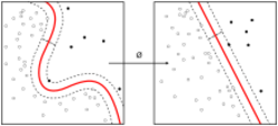
Kernel methods are popular in machine learning as they give the algorithm designed the freedom to design a "feature space" in which to measure the similarity of their data points. A simple kernel-based binary classifier is based on the following computation:

[math]\displaystyle{ \hat{y}(\mathbf{x'}) = \sgn \sum_{i=1}^n y_i k(\mathbf{x}_i, \mathbf{x'}), }[/math]

where [math]\displaystyle{ \mathbf{x}_i\in\mathbb{R}^d }[/math] are the data points, [math]\displaystyle{ y_i }[/math] is the label of the [math]\displaystyle{ i }[/math]th point (either −1 or +1), and [math]\displaystyle{ \hat{y}(\mathbf{x'}) }[/math] is the prediction of the class of [math]\displaystyle{ \mathbf{x'} }[/math]. The function [math]\displaystyle{ k : \mathbb{R}^d \times \mathbb R^d \to \mathbb R }[/math] is the kernel. Typical examples are the radial basis function kernel, [math]\displaystyle{ k(x,x') = \exp(-\|x-x'\|_2^2) }[/math], and polynomial kernels such as [math]\displaystyle{ k(x,x') = (1+\langle x, x'\rangle)^2 }[/math].

When used this way, the kernel method is called "implicit". Sometimes it is faster to do an "explicit" kernel method, in which a pair of functions [math]\displaystyle{ f, g : \mathbb{R}^d \to \mathbb{R}^D }[/math] are found, such that [math]\displaystyle{ k(x,x') = \langle f(x), g(x')\rangle }[/math]. This allows the above computation to be expressed as

[math]\displaystyle{ \hat{y}(\mathbf{x'}) = \sgn \sum_{i=1}^n y_i \langle f(\mathbf{x}_i), g(\mathbf{x'})\rangle = \sgn \left\langle\left(\sum_{i=1}^n y_i f(\mathbf{x}_i)\right), g(\mathbf{x'})\right\rangle, }[/math]

where the value [math]\displaystyle{ \sum_{i=1}^n y_i f(\mathbf{x}_i) }[/math] can be computed in advance.

The problem with this method is that the feature space can be very large. That is [math]\displaystyle{ D \gt \gt d }[/math]. For example, for the polynomial kernel [math]\displaystyle{ k(x,x') = \langle x,x'\rangle^3 }[/math] we get [math]\displaystyle{ f(x) = x\otimes x\otimes x }[/math] and [math]\displaystyle{ g(x') = x'\otimes x'\otimes x' }[/math], where [math]\displaystyle{ \otimes }[/math] is the tensor product and [math]\displaystyle{ f(x),g(x')\in\mathbb{R}^D }[/math] where [math]\displaystyle{ D=d^3 }[/math]. If [math]\displaystyle{ d }[/math] is already large, [math]\displaystyle{ D }[/math] can be much larger than the number of data points ([math]\displaystyle{ n }[/math]) and so the explicit method is inefficient.

The idea of tensor sketch is that we can compute approximate functions [math]\displaystyle{ f', g' : \mathbb R^d \to \mathbb R^t }[/math] where [math]\displaystyle{ t }[/math] can even be smaller than [math]\displaystyle{ d }[/math], and which still have the property that [math]\displaystyle{ \langle f'(x), g'(x')\rangle \approx k(x,x') }[/math].

This method was shown in 2020 to work even for high degree polynomials and radial basis function kernels.

Compressed matrix multiplication

Assume we have two large datasets, represented as matrices [math]\displaystyle{ X, Y\in\mathbb R^{n \times d} }[/math], and we want to find the rows [math]\displaystyle{ i,j }[/math] with the largest inner products [math]\displaystyle{ \langle X_i, Y_j\rangle }[/math]. We could compute [math]\displaystyle{ Z = X Y^T \in \mathbb R^{n\times n} }[/math] and simply look at all [math]\displaystyle{ n^2 }[/math] posibilities. However, this would take at least [math]\displaystyle{ n^2 }[/math] time, and probably closer to [math]\displaystyle{ n^2d }[/math] using standard matrix multiplication techniques.

The idea of Compressed Matrix Multiplication is the general identity

[math]\displaystyle{ X Y^T = \sum_{i=1}^d X_i \otimes Y_i }[/math]

where [math]\displaystyle{ \otimes }[/math] is the tensor product. Since we can compute a (linear) approximation to [math]\displaystyle{ X_i \otimes Y_i }[/math] efficiently, we can sum those up to get an approximation for the complete product.

Compact multilinear pooling

Tensor sketches can be used to decrease the number of variables needed when implementing Bilinear Pooling in a neural network.

Bilinear pooling is the technique of taking two input vectors, [math]\displaystyle{ x, y }[/math] from different sources, and using the tensor product [math]\displaystyle{ x\otimes y }[/math] as the input layer to a neural network.

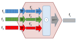
In the authors considered using tensor sketch to reduce the number of variables needed.

In 2017 another paper takes the FFT of the input features, before they are combined using the element-wise product. This again corresponds to the original tensor sketch.

References

- ↑ "Low-rank Tucker decomposition of large tensors using: Tensor Sketch". Boulder, Colorado: University of Colorado Boulder. https://amath.colorado.edu/faculty/becker/TensorSketch.pdf.
- ↑ Ahle, Thomas; Knudsen, Jakob (2019-09-03). "Almost Optimal Tensor Sketch". https://www.researchgate.net/publication/335617805_Almost_Optimal_Tensor_Sketch.
- ↑ 3.0 3.1 Woodruff, David P. "Sketching as a Tool for Numerical Linear Algebra." Theoretical Computer Science 10.1-2 (2014): 1–157.
- ↑ 4.0 4.1 Ninh, Pham; Rasmus, Pagh (2013). "Fast and scalable polynomial kernels via explicit feature maps". SIGKDD international conference on Knowledge discovery and data mining. Association for Computing Machinery. doi:10.1145/2487575.2487591.
- ↑ Rasmus, Pagh (2013). "Compressed matrix multiplication". ACM Transactions on Computation Theory, August 2013 Article No.: 9 (Association for Computing Machinery). doi:10.1145/2493252.2493254.
- ↑ Kasiviswanathan, Shiva Prasad, et al. "The price of privately releasing contingency tables and the spectra of random matrices with correlated rows." Proceedings of the forty-second ACM symposium on Theory of computing. 2010.
- ↑ Rudelson, Mark, and Shuheng Zhou. "Reconstruction from anisotropic random measurements." Conference on Learning Theory. 2012.
- ↑ Avron, Haim; Nguyen, Huy; Woodruff, David (2013). "Subspace Embeddings for the Polynomial Kernel". NIPS'14: Proceedings of the 27th International Conference on Neural Information Processing Systems (Association for Computing Machinery). doi:10.1145/2493252.2493254.
- ↑ 9.0 9.1 9.2 9.3 9.4 9.5 Ahle, Thomas; Kapralov, Michael; Knudsen, Jakob; Pagh, Rasmus; Velingker, Ameya; Woodruff, David; Zandieh, Amir (2020). "Oblivious Sketching of High-Degree Polynomial Kernels". ACM-SIAM Symposium on Discrete Algorithms. Association for Computing Machinery. doi:10.1137/1.9781611975994.9.
- ↑ Ailon, Nir; Chazelle, Bernard (2006). "Proceedings of the 38th Annual ACM Symposium on Theory of Computing". Proceedings of the 38th Annual ACM Symposium on Theory of Computing. New York: ACM Press. pp. 557–563. doi:10.1145/1132516.1132597. ISBN 1-59593-134-1.
- ↑ Jin, Ruhui, Tamara G. Kolda, and Rachel Ward. "Faster Johnson–Lindenstrauss Transforms via Kronecker Products." arXiv preprint arXiv:1909.04801 (2019).
- ↑ Wang, Yining; Tung, Hsiao-Yu; Smola, Alexander; Anandkumar, Anima. "Fast and Guaranteed Tensor Decomposition via Sketching". Advances in Neural Information Processing Systems 28 (NIPS 2015).
- ↑ Gao, Yang, et al. "Compact bilinear pooling." Proceedings of the IEEE conference on computer vision and pattern recognition. 2016.
- ↑ Algashaam, Faisal M., et al. "Multispectral periocular classification with multimodal compact multi-linear pooling." IEEE Access 5 (2017): 14572–14578.