Bernoulli distribution

Short description: Probability distribution modeling a coin toss which need not be fair

Bernoulli distribution

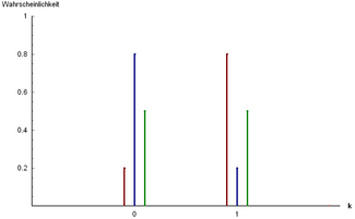
Probability mass function Three examples of Bernoulli distribution:   [math]\displaystyle{ P(x=0) = 0{.}2 }[/math] and [math]\displaystyle{ P(x=1) = 0{.}8 }[/math]   [math]\displaystyle{ P(x=0) = 0{.}8 }[/math] and [math]\displaystyle{ P(x=1) = 0{.}2 }[/math]   [math]\displaystyle{ P(x=0) = 0{.}5 }[/math] and [math]\displaystyle{ P(x=1) = 0{.}5 }[/math]
Parameters	[math]\displaystyle{ 0 \leq p \leq 1 }[/math] [math]\displaystyle{ q = 1 - p }[/math]
Support	[math]\displaystyle{ k \in \{0,1\} }[/math]
pmf	[math]\displaystyle{ \begin{cases} q=1-p & \text{if }k=0 \\ p & \text{if }k=1 \end{cases} }[/math]
CDF	[math]\displaystyle{ \begin{cases} 0 & \text{if } k \lt 0 \\ 1 - p & \text{if } 0 \leq k \lt 1 \\ 1 & \text{if } k \geq 1 \end{cases} }[/math]
Mean	[math]\displaystyle{ p }[/math]
Median	[math]\displaystyle{ \begin{cases} 0 & \text{if } p \lt 1/2\\ \left[0, 1\right] & \text{if } p = 1/2\\ 1 & \text{if } p \gt 1/2 \end{cases} }[/math]
Mode	[math]\displaystyle{ \begin{cases} 0 & \text{if } p \lt 1/2\\ 0, 1 & \text{if } p = 1/2\\ 1 & \text{if } p \gt 1/2 \end{cases} }[/math]
Variance	[math]\displaystyle{ p(1-p) = pq }[/math]
Skewness	[math]\displaystyle{ \frac{q - p}{\sqrt{pq}} }[/math]
Kurtosis	[math]\displaystyle{ \frac{1 - 6pq}{pq} }[/math]
Entropy	[math]\displaystyle{ -q\ln q - p\ln p }[/math]
MGF	[math]\displaystyle{ q+pe^t }[/math]
CF	[math]\displaystyle{ q+pe^{it} }[/math]
PGF	[math]\displaystyle{ q+pz }[/math]
Fisher information	[math]\displaystyle{ \frac{1}{pq} }[/math]

In probability theory and statistics, the Bernoulli distribution, named after Swiss mathematician Jacob Bernoulli, is the discrete probability distribution of a random variable which takes the value 1 with probability [math]\displaystyle{ p }[/math] and the value 0 with probability [math]\displaystyle{ q = 1-p }[/math]. Less formally, it can be thought of as a model for the set of possible outcomes of any single experiment that asks a yes–no question. Such questions lead to outcomes that are boolean-valued: a single bit whose value is success/yes/true/one with probability p and failure/no/false/zero with probability q. It can be used to represent a (possibly biased) coin toss where 1 and 0 would represent "heads" and "tails", respectively, and p would be the probability of the coin landing on heads (or vice versa where 1 would represent tails and p would be the probability of tails). In particular, unfair coins would have [math]\displaystyle{ p \neq 1/2. }[/math]

The Bernoulli distribution is a special case of the binomial distribution where a single trial is conducted (so n would be 1 for such a binomial distribution). It is also a special case of the two-point distribution, for which the possible outcomes need not be 0 and 1.

Properties

If [math]\displaystyle{ X }[/math] is a random variable with a Bernoulli distribution, then:

[math]\displaystyle{ \Pr(X=1) = p = 1 - \Pr(X=0) = 1 - q. }[/math]

The probability mass function [math]\displaystyle{ f }[/math] of this distribution, over possible outcomes k, is

[math]\displaystyle{ f(k;p) = \begin{cases} p & \text{if }k=1, \\ q = 1-p & \text {if } k = 0. \end{cases} }[/math]

This can also be expressed as

[math]\displaystyle{ f(k;p) = p^k (1-p)^{1-k} \quad \text{for } k\in\{0,1\} }[/math]

or as

[math]\displaystyle{ f(k;p)=pk+(1-p)(1-k) \quad \text{for } k\in\{0,1\}. }[/math]

The Bernoulli distribution is a special case of the binomial distribution with [math]\displaystyle{ n = 1. }[/math]

The kurtosis goes to infinity for high and low values of [math]\displaystyle{ p, }[/math] but for [math]\displaystyle{ p=1/2 }[/math] the two-point distributions including the Bernoulli distribution have a lower excess kurtosis, namely −2, than any other probability distribution.

The Bernoulli distributions for [math]\displaystyle{ 0 \le p \le 1 }[/math] form an exponential family.

The maximum likelihood estimator of [math]\displaystyle{ p }[/math] based on a random sample is the sample mean.

The probability mass distribution function of a Bernoulli experiment along with its corresponding cumulative distribution function.

Mean

The expected value of a Bernoulli random variable [math]\displaystyle{ X }[/math] is

[math]\displaystyle{ \operatorname{E}[X]=p }[/math]

This is due to the fact that for a Bernoulli distributed random variable [math]\displaystyle{ X }[/math] with [math]\displaystyle{ \Pr(X=1)=p }[/math] and [math]\displaystyle{ \Pr(X=0)=q }[/math] we find

[math]\displaystyle{ \operatorname{E}[X] = \Pr(X=1)\cdot 1 + \Pr(X=0)\cdot 0 = p \cdot 1 + q\cdot 0 = p. }[/math]

Variance

The variance of a Bernoulli distributed [math]\displaystyle{ X }[/math] is

[math]\displaystyle{ \operatorname{Var}[X] = pq = p(1-p) }[/math]

We first find

[math]\displaystyle{ \operatorname{E}[X^2] = \Pr(X=1)\cdot 1^2 + \Pr(X=0)\cdot 0^2 = p \cdot 1^2 + q\cdot 0^2 = p = \operatorname{E}[X] }[/math]

From this follows

[math]\displaystyle{ \operatorname{Var}[X] = \operatorname{E}[X^2]-\operatorname{E}[X]^2 = \operatorname{E}[X]-\operatorname{E}[X]^2 = p-p^2 = p(1-p) = pq }[/math]

With this result it is easy to prove that, for any Bernoulli distribution, its variance will have a value inside [math]\displaystyle{ [0,1/4] }[/math].

Skewness

The skewness is [math]\displaystyle{ \frac{q-p}{\sqrt{pq}}=\frac{1-2p}{\sqrt{pq}} }[/math]. When we take the standardized Bernoulli distributed random variable [math]\displaystyle{ \frac{X-\operatorname{E}[X]}{\sqrt{\operatorname{Var}[X]}} }[/math] we find that this random variable attains [math]\displaystyle{ \frac{q}{\sqrt{pq}} }[/math] with probability [math]\displaystyle{ p }[/math] and attains [math]\displaystyle{ -\frac{p}{\sqrt{pq}} }[/math] with probability [math]\displaystyle{ q }[/math]. Thus we get

[math]\displaystyle{ \begin{align} \gamma_1 &= \operatorname{E} \left[\left(\frac{X-\operatorname{E}[X]}{\sqrt{\operatorname{Var}[X]}}\right)^3\right] \\ &= p \cdot \left(\frac{q}{\sqrt{pq}}\right)^3 + q \cdot \left(-\frac{p}{\sqrt{pq}}\right)^3 \\ &= \frac{1}{\sqrt{pq}^3} \left(pq^3-qp^3\right) \\ &= \frac{pq}{\sqrt{pq}^3} (q-p) \\ &= \frac{q-p}{\sqrt{pq}}. \end{align} }[/math]

Higher moments and cumulants

The raw moments are all equal due to the fact that [math]\displaystyle{ 1^k=1 }[/math] and [math]\displaystyle{ 0^k=0 }[/math].

[math]\displaystyle{ \operatorname{E}[X^k] = \Pr(X=1)\cdot 1^k + \Pr(X=0)\cdot 0^k = p \cdot 1 + q\cdot 0 = p = \operatorname{E}[X]. }[/math]

The central moment of order [math]\displaystyle{ k }[/math] is given by

[math]\displaystyle{ \mu_k =(1-p)(-p)^k +p(1-p)^k. }[/math]

The first six central moments are

[math]\displaystyle{ \begin{align} \mu_1 &= 0, \\ \mu_2 &= p(1-p), \\ \mu_3 &= p(1-p)(1-2p), \\ \mu_4 &= p(1-p)(1-3p(1-p)), \\ \mu_5 &= p(1-p)(1-2p)(1-2p(1-p)), \\ \mu_6 &= p(1-p)(1-5p(1-p)(1-p(1-p))). \end{align} }[/math]

The higher central moments can be expressed more compactly in terms of [math]\displaystyle{ \mu_2 }[/math] and [math]\displaystyle{ \mu_3 }[/math]

[math]\displaystyle{ \begin{align} \mu_4 &= \mu_2 (1-3\mu_2 ), \\ \mu_5 &= \mu_3 (1-2\mu_2 ), \\ \mu_6 &= \mu_2 (1-5\mu_2 (1-\mu_2 )). \end{align} }[/math]

The first six cumulants are

[math]\displaystyle{ \begin{align} \kappa_1 &= p, \\ \kappa_2 &= \mu_2 , \\ \kappa_3 &= \mu_3 , \\ \kappa_4 &= \mu_2 (1-6\mu_2 ), \\ \kappa_5 &= \mu_3 (1-12\mu_2 ), \\ \kappa_6 &= \mu_2 (1-30\mu_2 (1-4\mu_2 )). \end{align} }[/math]

Related distributions

• If [math]\displaystyle{ X_1,\dots,X_n }[/math] are independent, identically distributed (i.i.d.) random variables, all Bernoulli trials with success probability p, then their sum is distributed according to a binomial distribution with parameters n and p:

  [math]\displaystyle{ \sum_{k=1}^n X_k \sim \operatorname{B}(n,p) }[/math] (binomial distribution).

The Bernoulli distribution is simply [math]\displaystyle{ \operatorname{B}(1, p) }[/math], also written as [math]\displaystyle{ \mathrm{Bernoulli} (p). }[/math]

• The categorical distribution is the generalization of the Bernoulli distribution for variables with any constant number of discrete values.
• The Beta distribution is the conjugate prior of the Bernoulli distribution.
• The geometric distribution models the number of independent and identical Bernoulli trials needed to get one success.
• If [math]\displaystyle{ Y \sim \mathrm{Bernoulli}\left(\frac{1}{2}\right) }[/math], then [math]\displaystyle{ 2Y - 1 }[/math] has a Rademacher distribution.

See also

• Bernoulli process, a random process consisting of a sequence of independent Bernoulli trials
• Bernoulli sampling
• Binary entropy function
• Binary decision diagram

Further reading

• Johnson, N. L.; Kotz, S.; Kemp, A. (1993). Univariate Discrete Distributions (2nd ed.). Wiley. ISBN 0-471-54897-9. 
• Peatman, John G. (1963). Introduction to Applied Statistics. New York: Harper & Row. pp. 162–171. 

External links

• Hazewinkel, Michiel, ed. (2001), "Binomial distribution", Encyclopedia of Mathematics, Springer Science+Business Media B.V. / Kluwer Academic Publishers, ISBN 978-1-55608-010-4, https://www.encyclopediaofmath.org/index.php?title=p/b016420 .
• Weisstein, Eric W.. "Bernoulli Distribution". http://mathworld.wolfram.com/BernoulliDistribution.html. 
• Interactive graphic: Univariate Distribution Relationships.

References

- ↑ Uspensky, James Victor (1937). Introduction to Mathematical Probability. New York: McGraw-Hill. p. 45. OCLC 996937.
- ↑ Dekking, Frederik; Kraaikamp, Cornelis; Lopuhaä, Hendrik; Meester, Ludolf (9 October 2010). A Modern Introduction to Probability and Statistics (1 ed.). Springer London. pp. 43–48. ISBN 9781849969529.
- ↑ 3.0 3.1 3.2 3.3 Bertsekas, Dimitri P. (2002). Introduction to Probability. Tsitsiklis, John N., Τσιτσικλής, Γιάννης Ν.. Belmont, Mass.: Athena Scientific. ISBN 188652940X. OCLC 51441829.
- ↑ McCullagh, Peter; Nelder, John (1989). Generalized Linear Models, Second Edition. Boca Raton: Chapman and Hall/CRC. Section 4.2.2. ISBN 0-412-31760-5.
- ↑ Orloff, Jeremy; Bloom, Jonathan. "Conjugate priors: Beta and normal". https://math.mit.edu/~dav/05.dir/class15-prep.pdf.