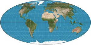
Equal-area projection

Short description: Type of map projection

The equal-area Mollweide projection

In cartography, an equivalent, authalic, or equal-area projection is a map projection that preserves relative area measure between any and all map regions. Equivalent projections are widely used for thematic maps showing scenario distribution such as population, farmland distribution, forested areas, and so forth, because an equal-area map does not change apparent density of the phenomenon being mapped.

By Gauss's Theorema Egregium, an equal-area projection cannot be conformal. This implies that an equal-area projection inevitably distorts shapes. Even though a point or points or a path or paths on a map might have no distortion, the greater the area of the region being mapped, the greater and more obvious the distortion of shapes inevitably becomes.

Lambert azimuthal equal-area projection of the world centered on 0° N 0° E.

Description

In order for a map projection of the sphere to be equal-area, its generating formulae must meet this Cauchy-Riemann-like condition:

[math]\displaystyle{ \frac{\partial y}{\partial \varphi} \cdot \frac{\partial x}{\partial \lambda} - \frac{\partial y}{\partial \lambda} \cdot \frac{\partial x}{\partial \varphi} = s \cdot \cos \varphi }[/math]

where [math]\displaystyle{ s }[/math] is constant throughout the map. Here, [math]\displaystyle{ \varphi }[/math] represents latitude; [math]\displaystyle{ \lambda }[/math] represents longitude; and [math]\displaystyle{ x }[/math] and [math]\displaystyle{ y }[/math] are the projected (planar) coordinates for a given [math]\displaystyle{ (\varphi, \lambda) }[/math] coordinate pair.

For example, the sinusoidal projection is a very simple equal-area projections. Its generating formulæ are:

[math]\displaystyle{ \begin{align} x &= R \cdot \lambda \cos \varphi \\ y &= R \cdot \varphi \end{align} }[/math]

where [math]\displaystyle{ R }[/math] is the radius of the globe. Computing the partial derivatives,

[math]\displaystyle{ \frac{\partial x}{\partial \varphi} = -R \cdot \lambda \cdot \sin \varphi,\quad R \cdot \frac{\partial x}{\partial \lambda} = R \cdot \cos \varphi,\quad \frac{\partial y}{\partial \varphi} = R,\quad \frac{\partial y}{\partial \lambda} = 0 }[/math]

and so

[math]\displaystyle{ \frac{\partial y}{\partial \varphi} \cdot \frac{\partial x}{\partial \lambda} - \frac{\partial y}{\partial \lambda} \cdot \frac{\partial x}{\partial \varphi} = R \cdot R \cdot \cos \varphi - 0 \cdot (-R \cdot \lambda \cdot \sin \varphi) = R^2 \cdot \cos \varphi = s \cdot \cos \varphi }[/math]

with [math]\displaystyle{ s }[/math] taking the value of the constant [math]\displaystyle{ R^2 }[/math].

For an equal-area map of the ellipsoid, the corresponding differential condition that must be met is:

[math]\displaystyle{ \frac{\partial y}{\partial \varphi} \cdot \frac{\partial x}{\partial \lambda} - \frac{\partial y}{\partial \lambda} \cdot \frac{\partial x}{\partial \varphi} = s \cdot \cos \varphi \cdot \frac{(1-e^2)}{(1-e^2 \sin^2 \varphi)^2} }[/math]

where [math]\displaystyle{ e }[/math] is the eccentricity of the ellipsoid of revolution.

Statistical grid

The term "statistical grid" refers to a discrete grid (global or local) of an equal-area surface representation, used for data visualization, geocode and statistical spatial analysis.

List of equal-area projections

These are some projections that preserve area:

• Azimuthal
  • Lambert azimuthal equal-area
  • Wiechel (pseudoazimuthal)

Albers projection of the world with standard parallels 20° N and 50° N.

• Conic
  • Albers
  • Lambert equal-area conic projection

Bottomley projection of the world with standard parallel at 30° N.

• Pseudoconical
  • Bonne
  • Bottomley
  • Werner

Lambert cylindrical equal-area projection of the world

• Cylindrical (with latitude of no distortion)
  • Lambert cylindrical equal-area (0°)
  • Behrmann (30°)
  • Hobo–Dyer (37°30′)
  • Gall–Peters (45°)

Equal Earth projection, an equal-area pseudocylindrical projection

• Pseudocylindrical
  • Boggs eumorphic
  • Collignon
  • Eckert II, IV and VI
  • Equal Earth
  • Goode's homolosine
  • Mollweide
  • Sinusoidal
  • Tobler hyperelliptical
• Other
  • Eckert-Greifendorff
  • McBryde-Thomas Flat-Polar Quartic Projection
  • Hammer
  • Strebe 1995
  • Snyder equal-area projection, used for geodesic grids.

See also

• Authalic latitude
• Authalic radius
• Equiareal map (mathematics)
• Measure-preserving dynamical system
• Geodesic polygon area

References

- ↑ 1.0 1.1 Snyder, John P. (1987). Map projections — A working manual. USGS Professional Paper. 1395. Washington: United States Government Printing Office. p. 28. doi:10.3133/pp1395. https://pubs.er.usgs.gov/publication/pp1395.
- ↑ "INSPIRE helpdesk | INSPIRE". https://inspire.ec.europa.eu/forum/discussion/view/10928/use-of-the-equal-area-grid-grid-etrs89-laea.
- ↑ http://scorus.org/wp-content/uploads/2012/10/2010JurmalaP4.5.pdf[|permanent dead link|dead link}}]
- ↑ IBGE (2016), "Grade Estatística". Arquivo
grade_estatistica.pdfem FTP ou HTTP, Censo 2010[|permanent dead link|dead link}}] - ↑ Tsoulos, Lysandros (2003). "An Equal Area Projection for Statistical Mapping in the EU". Map projections for Europe. Joint Research Centre, European Commission. pp. 50–55. https://www.researchgate.net/publication/236852866.
- ↑ Brodzik, Mary J.; Billingsley, Brendan; Haran, Terry; Raup, Bruce; Savoie, Matthew H. (2012-03-13). "EASE-Grid 2.0: Incremental but Significant Improvements for Earth-Gridded Data Sets". ISPRS International Journal of Geo-Information (MDPI AG) 1 (1): 32–45. doi:10.3390/ijgi1010032. ISSN 2220-9964.
- ↑ "McBryde-Thomas Flat-Polar Quartic Projection - MATLAB". https://www.mathworks.com/help/map/flatplrq.html. Retrieved 3 January 2024.