Boltzmann machine

A Boltzmann machine (also called Sherrington–Kirkpatrick model with external field or stochastic Ising model), named after Ludwig Boltzmann, is a spin-glass model with an external field, i.e., a Sherrington–Kirkpatrick model,[1] that is a stochastic Ising model. It is a statistical physics technique applied in the context of cognitive science.[2] It is also classified as a Markov random field.[3]
Boltzmann machines are theoretically intriguing because of the locality and Hebbian nature of their training algorithm (being trained by Hebb's rule), and because of their parallelism and the resemblance of their dynamics to simple physical processes. Boltzmann machines with unconstrained connectivity have not been proven useful for practical problems in machine learning or inference, but if the connectivity is properly constrained, the learning can be made efficient enough to be useful for practical problems.[4]
They are named after the Boltzmann distribution in statistical mechanics, which is used in their sampling function. They were heavily popularized and promoted by Geoffrey Hinton, Terry Sejnowski and Yann LeCun in cognitive sciences communities, particularly in machine learning,[2] as part of "energy-based models" (EBM), because Hamiltonians of spin glasses as energy are used as a starting point to define the learning task.[5]
Structure

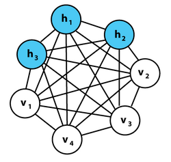
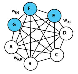
A Boltzmann machine, like a Sherrington–Kirkpatrick model, is a network of units with a total "energy" (Hamiltonian) defined for the overall network. Its units produce binary results. Boltzmann machine weights are stochastic. The global energy in a Boltzmann machine is identical in form to that of Hopfield networks and Ising models:
Where:
- is the connection strength between unit and unit .
- is the state, , of unit .
- is the bias of unit in the global energy function. ( is the activation threshold for the unit.)
Often the weights are represented as a symmetric matrix with zeros along the diagonal.
Unit state probability
The difference in the global energy that results from a single unit equaling 0 (off) versus 1 (on), written , assuming a symmetric matrix of weights, is given by:
This can be expressed as the difference of energies of two states:
Substituting the energy of each state with its relative probability according to the Boltzmann factor (the property of a Boltzmann distribution that the energy of a state is proportional to the negative log probability of that state) yields:
where is the Boltzmann constant and is absorbed into the artificial notion of temperature . Noting that the probabilities of the unit being on or off sum to allows for the simplification:
whence the probability that the -th unit is given by
where the scalar is referred to as the temperature of the system. This relation is the source of the logistic function found in probability expressions in variants of the Boltzmann machine.
Equilibrium state
The network runs by repeatedly choosing a unit and resetting its state. After running for long enough at a certain temperature, the probability of a global state of the network depends only upon that global state's energy, according to a Boltzmann distribution, and not on the initial state from which the process was started. This means that log-probabilities of global states become linear in their energies. This relationship is true when the machine is "at thermal equilibrium", meaning that the probability distribution of global states has converged. Running the network beginning from a high temperature, its temperature gradually decreases until reaching a thermal equilibrium at a lower temperature. It then may converge to a distribution where the energy level fluctuates around the global minimum. This process is called simulated annealing.
To train the network so that the chance it will converge to a global state according to an external distribution over these states, the weights must be set so that the global states with the highest probabilities get the lowest energies. This is done by training.
Training
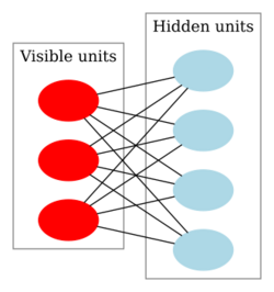
The units in the Boltzmann machine are divided into 'visible' units, V, and 'hidden' units, H. The visible units are those that receive information from the 'environment', i.e. the training set is a set of binary vectors over the set V. The distribution over the training set is denoted .
The distribution over global states converges as the Boltzmann machine reaches thermal equilibrium. We denote this distribution, after we marginalize it over the hidden units, as .
Our goal is to approximate the "real" distribution using the produced by the machine. The similarity of the two distributions is measured by the Kullback–Leibler divergence, :
where the sum is over all the possible states of . is a function of the weights, since they determine the energy of a state, and the energy determines , as promised by the Boltzmann distribution. A gradient descent algorithm over changes a given weight, , by subtracting the partial derivative of with respect to the weight.
Boltzmann machine training involves two alternating phases. One is the "positive" phase where the visible units' states are clamped to a particular binary state vector sampled from the training set (according to ). The other is the "negative" phase where the network is allowed to run freely, i.e. only the input nodes have their state determined by external data, but the output nodes are allowed to float. The gradient with respect to a given weight, , is given by the equation:[2]
where:
- is the probability that units i and j are both on when the machine is at equilibrium on the positive phase.
- is the probability that units i and j are both on when the machine is at equilibrium on the negative phase.
- denotes the learning rate
This result follows from the fact that at thermal equilibrium the probability of any global state when the network is free-running is given by the Boltzmann distribution.
This learning rule is biologically plausible because the only information needed to change the weights is provided by "local" information. That is, the connection (synapse, biologically) does not need information about anything other than the two neurons it connects. This is more biologically realistic than the information needed by a connection in many other neural network training algorithms, such as backpropagation.
The training of a Boltzmann machine does not use the EM algorithm, which is heavily used in machine learning. By minimizing the KL-divergence, it is equivalent to maximizing the log-likelihood of the data. Therefore, the training procedure performs gradient ascent on the log-likelihood of the observed data. This is in contrast to the EM algorithm, where the posterior distribution of the hidden nodes must be calculated before the maximization of the expected value of the complete data likelihood during the M-step.
Training the biases is similar, but uses only single node activity:
Problems
Theoretically the Boltzmann machine is a rather general computational medium. For instance, if trained on photographs, the machine would theoretically model the distribution of photographs, and could use that model to, for example, complete a partial photograph.
Unfortunately, Boltzmann machines experience a serious practical problem, namely that it seems to stop learning correctly when the machine is scaled up to anything larger than a trivial size. This is due to important effects, specifically:
- connection strengths are more plastic when the connected units have activation probabilities intermediate between zero and one, leading to a so-called variance trap. The net effect is that noise causes the connection strengths to follow a random walk until the activities saturate.
Types
Restricted Boltzmann machine

Although learning is impractical in general Boltzmann machines, it can be made quite efficient in a restricted Boltzmann machine (RBM) which does not allow intralayer connections between hidden units and visible units, i.e. there is no connection between visible to visible and hidden to hidden units. After training one RBM, the activities of its hidden units can be treated as data for training a higher-level RBM. This method of stacking RBMs makes it possible to train many layers of hidden units efficiently and is one of the most common deep learning strategies. As each new layer is added the generative model improves.
An extension to the restricted Boltzmann machine allows using real valued data rather than binary data.[6]
One example of a practical RBM application is in speech recognition.[7]
Deep Boltzmann machine
A deep Boltzmann machine (DBM) is a type of binary pairwise Markov random field (undirected probabilistic graphical model) with multiple layers of hidden random variables. It is a network of symmetrically coupled stochastic binary units. It comprises a set of visible units and layers of hidden units . No connection links units of the same layer (like RBM). For the DBM, the probability assigned to vector ν is
where are the set of hidden units, and are the model parameters, representing visible-hidden and hidden-hidden interactions.[8] In a DBN only the top two layers form a restricted Boltzmann machine (which is an undirected graphical model), while lower layers form a directed generative model. In a DBM all layers are symmetric and undirected.
Like DBNs, DBMs can learn complex and abstract internal representations of the input in tasks such as object or speech recognition, using limited, labeled data to fine-tune the representations built using a large set of unlabeled sensory input data. However, unlike DBNs and deep convolutional neural networks, they pursue the inference and training procedure in both directions, bottom-up and top-down, which allow the DBM to better unveil the representations of the input structures.[9][10][11]
However, the slow speed of DBMs limits their performance and functionality. Because exact maximum likelihood learning is intractable for DBMs, only approximate maximum likelihood learning is possible. Another option is to use mean-field inference to estimate data-dependent expectations and approximate the expected sufficient statistics by using Markov chain Monte Carlo (MCMC).[8] This approximate inference, which must be done for each test input, is about 25 to 50 times slower than a single bottom-up pass in DBMs. This makes joint optimization impractical for large data sets, and restricts the use of DBMs for tasks such as feature representation.
Spike-and-slab RBMs
The need for deep learning with real-valued inputs, as in Gaussian RBMs, led to the spike-and-slab RBM (ssRBM), which models continuous-valued inputs with binary latent variables.[12] Similar to basic RBMs and its variants, a spike-and-slab RBM is a bipartite graph, while like GRBMs, the visible units (input) are real-valued. The difference is in the hidden layer, where each hidden unit has a binary spike variable and a real-valued slab variable. A spike is a discrete probability mass at zero, while a slab is a density over continuous domain;[13] their mixture forms a prior.[14]
An extension of ssRBM called μ-ssRBM provides extra modeling capacity using additional terms in the energy function. One of these terms enables the model to form a conditional distribution of the spike variables by marginalizing out the slab variables given an observation.
In mathematics
In more general mathematical setting, the Boltzmann distribution is also known as the Gibbs measure. In statistics and machine learning it is called a log-linear model. In deep learning the Boltzmann distribution is used in the sampling distribution of stochastic neural networks such as the Boltzmann machine.
History
The Boltzmann machine is based on the Sherrington–Kirkpatrick spin glass model by David Sherrington and Scott Kirkpatrick.[15] The seminal publication by John Hopfield (1982) applied methods of statistical mechanics, mainly the recently developed (1970s) theory of spin glasses, to study associative memory (later named the "Hopfield network").[16]
The original contribution in applying such energy-based models in cognitive science appeared in papers by Geoffrey Hinton and Terry Sejnowski.[17][18][19] In a 1995 interview, Hinton stated that in 1983 February or March, he was going to give a talk on simulated annealing in Hopfield networks, so he had to design a learning algorithm for the talk, resulting in the Boltzmann machine learning algorithm.[20]
The idea of applying the Ising model with annealed Gibbs sampling was used in Douglas Hofstadter's Copycat project (1984).[21][22]
The explicit analogy drawn with statistical mechanics in the Boltzmann machine formulation led to the use of terminology borrowed from physics (e.g., "energy"), which became standard in the field. The widespread adoption of this terminology may have been encouraged by the fact that its use led to the adoption of a variety of concepts and methods from statistical mechanics. The various proposals to use simulated annealing for inference were apparently independent.
Similar ideas (with a change of sign in the energy function) are found in Paul Smolensky's "Harmony Theory".[23] Ising models can be generalized to Markov random fields, which find widespread application in linguistics, robotics, computer vision and artificial intelligence.
In 2024, Hopfield and Hinton were awarded Nobel Prize in Physics for their foundational contributions to machine learning, such as the Boltzmann machine.[24]
See also
- Restricted Boltzmann machine
- Helmholtz machine
- Markov random field (MRF)
- Ising model (Lenz–Ising model)
- Hopfield network
References
- ↑ Sherrington, David; Kirkpatrick, Scott (1975), "Solvable Model of a Spin-Glass", Physical Review Letters 35 (35): 1792–1796, doi:10.1103/PhysRevLett.35.1792, Bibcode: 1975PhRvL..35.1792S
- ↑ 2.0 2.1 2.2 Ackley, David H.; Hinton, Geoffrey E.; Sejnowski, Terrence J. (1985). "A Learning Algorithm for Boltzmann Machines". Cognitive Science 9 (1): 147–169. doi:10.1207/s15516709cog0901_7. http://learning.cs.toronto.edu/~hinton/absps/cogscibm.pdf.
- ↑ Hinton, Geoffrey E. (2007-05-24). "Boltzmann machine" (in en). Scholarpedia 2 (5): 1668. doi:10.4249/scholarpedia.1668. ISSN 1941-6016. Bibcode: 2007SchpJ...2.1668H.
- ↑ Osborn, Thomas R. (1 January 1990). "Fast Teaching of Boltzmann Machines with Local Inhibition". International Neural Network Conference. Springer Netherlands. pp. 785. doi:10.1007/978-94-009-0643-3_76. ISBN 978-0-7923-0831-7. https://archive.org/details/innc90parisinter0001inte/page/785.
- ↑ Nijkamp, E.; Hill, M. E; Han, T. (2020), "On the Anatomy of MCMC-Based Maximum Likelihood Learning of Energy-Based Models", Proceedings of the AAAI Conference on Artificial Intelligence 4 (34): 5272–5280, doi:10.1609/aaai.v34i04.5973, https://ojs.aaai.org/index.php/AAAI/article/view/5973
- ↑ (in en) Recent Developments in Deep Learning, 22 March 2010, https://www.youtube.com/watch?v=VdIURAu1-aU, retrieved 2020-02-17
- ↑ Yu, Dong; Dahl, George; Acero, Alex; Deng, Li (2011). "Context-Dependent Pre-trained Deep Neural Networks for Large Vocabulary Speech Recognition". Microsoft Research 20. http://research.microsoft.com/pubs/144412/DBN4LVCSR-TransASLP.pdf.
- ↑ 8.0 8.1 Hinton, Geoffrey; Salakhutdinov, Ruslan (2012). "A better way to pretrain deep Boltzmann machines". Advances in Neural 3: 1–9. http://machinelearning.wustl.edu/mlpapers/paper_files/NIPS2012_1178.pdf. Retrieved 2017-08-18.
- ↑ Hinton, Geoffrey; Salakhutdinov, Ruslan (2009). "Efficient Learning of Deep Boltzmann Machines". 3. pp. 448–455. http://machinelearning.wustl.edu/mlpapers/paper_files/AISTATS09_SalakhutdinovH.pdf. Retrieved 2017-08-18.
- ↑ Bengio, Yoshua; LeCun, Yann (2007). "Scaling Learning Algorithms towards AI". http://www.iro.umontreal.ca/~lisa/bib/pub_subject/language/pointeurs/bengio+lecun-chapter2007.pdf.
- ↑ Larochelle, Hugo; Salakhutdinov, Ruslan (2010). "Efficient Learning of Deep Boltzmann Machines". pp. 693–700. http://machinelearning.wustl.edu/mlpapers/paper_files/AISTATS2010_SalakhutdinovL10.pdf. Retrieved 2017-08-18.
- ↑ Courville, Aaron; Bergstra, James; Bengio, Yoshua (2011). "A Spike and Slab Restricted Boltzmann Machine". JMLR: Workshop and Conference Proceeding 15: 233–241. http://machinelearning.wustl.edu/mlpapers/paper_files/AISTATS2011_CourvilleBB11.pdf. Retrieved 2019-08-25.
- ↑ Courville, Aaron; Bergstra, James; Bengio, Yoshua (2011). "Proceedings of the 28th International Conference on Machine Learning". 10. pp. 1–8.
- ↑ Mitchell, T; Beauchamp, J (1988). "Bayesian Variable Selection in Linear Regression". Journal of the American Statistical Association 83 (404): 1023–1032. doi:10.1080/01621459.1988.10478694.
- ↑ Sherrington, David; Kirkpatrick, Scott (1975-12-29). "Solvable Model of a Spin-Glass". Physical Review Letters 35 (26): 1792–1796. doi:10.1103/physrevlett.35.1792. ISSN 0031-9007. Bibcode: 1975PhRvL..35.1792S.
- ↑ Hopfield, J. J. (1982). "Neural networks and physical systems with emergent collective computational abilities". Proceedings of the National Academy of Sciences of the United States of America ([s.n.]) 79 (8): 2554–8. doi:10.1073/pnas.79.8.2554. OCLC 848771572. PMID 6953413. Bibcode: 1982PNAS...79.2554H.
- ↑ Hinton, Geoffery; Sejnowski, Terrence J. (May 1983). "Analyzing Cooperative Computation". 5th Annual Congress of the Cognitive Science Society. Rochester, New York. http://digitalcollections.library.cmu.edu/awweb/awarchive?type=file&item=360445. Retrieved 17 February 2020.
- ↑ Hinton, Geoffrey E.; Sejnowski, Terrence J. (June 1983). "Optimal Perceptual Inference". IEEE Conference on Computer Vision and Pattern Recognition (CVPR). Washington, D.C.: IEEE Computer Society. pp. 448–453.
- ↑ Fahlman SE, Hinton GE, Sejnowski TJ. Massively parallel architectures for Al: NETL, Thistle, and Boltzmann machines. In: Genesereth MR, editor. AAAI-83. Washington, DC: AAAI; 1983. pp. 109–113
- ↑ Chapter 16. Rosenfeld, Edward, and James A. Anderson, eds. 2000. Talking Nets: An Oral History of Neural Networks. Reprint edition. The MIT Press.
- ↑ Hofstadter, D. R. (January 1984). The Copycat Project: An Experiment in Nondeterminism and Creative Analogies.. Defense Technical Information Center. OCLC 227617764.
- ↑ Hofstadter, Douglas R. (1988). "A Non-Deterministic Approach to Analogy, Involving the Ising Model of Ferromagnetism". in Caianiello, Eduardo R.. Physics of cognitive processes. Teaneck, New Jersey: World Scientific. ISBN 9971-5-0255-0. OCLC 750950619.
- ↑ Smolensky, Paul. "Information processing in dynamical systems: Foundations of harmony theory." (1986): 194-281.
- ↑ Johnston, Hamish (2024-10-08). "John Hopfield and Geoffrey Hinton share the 2024 Nobel Prize for Physics" (in en-GB). https://physicsworld.com/a/john-hopfield-and-geoffrey-hinton-share-the-2024-nobel-prize-for-physics/.
Further reading
- Hinton, G. E.; Sejnowski, T. J. (1986). D. E. Rumelhart. ed. "Learning and Relearning in Boltzmann Machines". Parallel Distributed Processing: Explorations in the Microstructure of Cognition. Volume 1: Foundations: 282–317. http://www.cs.toronto.edu/~hinton/absps/pdp7.pdf.
- "Training Products of Experts by Minimizing Contrastive Divergence". Neural Computation 14 (8): 1771–1800. 2002. doi:10.1162/089976602760128018. PMID 12180402. http://www.cs.toronto.edu/~hinton/absps/nccd.pdf.
- "A fast learning algorithm for deep belief nets". Neural Computation 18 (7): 1527–1554. 2006. doi:10.1162/neco.2006.18.7.1527. PMID 16764513. http://www.cs.toronto.edu/~hinton/absps/fastnc.pdf.
- Kothari P (2020): https://www.forbes.com/sites/tomtaulli/2020/02/02/coronavirus-can-ai-artificial-intelligence-make-a-difference/?sh=1eca51e55817
- Montufar, Guido (2018). "Restricted Boltzmann Machines: Introduction and Review" (in en). https://www.mis.mpg.de/preprints/2018/preprint2018_87.pdf.
External links
 |
