Projection matrix

Short description: Concept in statistics

In statistics, the projection matrix [math]\displaystyle{ (\mathbf{P}) }[/math], sometimes also called the influence matrix or hat matrix [math]\displaystyle{ (\mathbf{H}) }[/math], maps the vector of response values (dependent variable values) to the vector of fitted values (or predicted values). It describes the influence each response value has on each fitted value.

[math]\displaystyle{ p_{ij} = \frac{\operatorname{Cov}\left[ \hat{y}_i, y_j \right]}{\operatorname{Var}\left[y_j \right]} }[/math]

Application for residuals

The formula for the vector of residuals [math]\displaystyle{ \mathbf{r} }[/math] can also be expressed compactly using the projection matrix:

[math]\displaystyle{ \mathbf{r} = \mathbf{y} - \mathbf{\hat{y}} = \mathbf{y} - \mathbf{P} \mathbf{y} = \left( \mathbf{I} - \mathbf{P} \right) \mathbf{y}. }[/math]

where [math]\displaystyle{ \mathbf{I} }[/math] is the identity matrix. The matrix [math]\displaystyle{ \mathbf{M} := \mathbf{I} - \mathbf{P} }[/math] is sometimes referred to as the residual maker matrix or the annihilator matrix.

The covariance matrix of the residuals [math]\displaystyle{ \mathbf{r} }[/math], by error propagation, equals

[math]\displaystyle{ \mathbf{\Sigma}_\mathbf{r} = \left( \mathbf{I} - \mathbf{P} \right)^\textsf{T} \mathbf{\Sigma} \left( \mathbf{I}-\mathbf{P} \right) }[/math],

where [math]\displaystyle{ \mathbf{\Sigma} }[/math] is the covariance matrix of the error vector (and by extension, the response vector as well). For the case of linear models with independent and identically distributed errors in which [math]\displaystyle{ \mathbf{\Sigma} = \sigma^{2} \mathbf{I} }[/math], this reduces to:

[math]\displaystyle{ \mathbf{\Sigma}_\mathbf{r} = \left( \mathbf{I} - \mathbf{P} \right) \sigma^{2} }[/math].

Intuition

A matrix, [math]\displaystyle{ \mathbf{A} }[/math] has its column space depicted as the green line. The projection of some vector [math]\displaystyle{ \mathbf{b} }[/math] onto the column space of [math]\displaystyle{ \mathbf{A} }[/math] is the vector [math]\displaystyle{ \mathbf{x} }[/math]

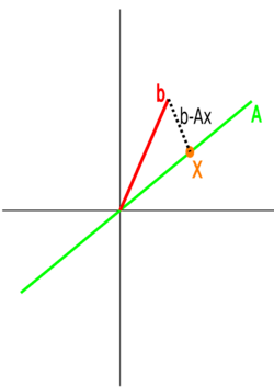
From the figure, it is clear that the closest point from the vector [math]\displaystyle{ \mathbf{b} }[/math] onto the column space of [math]\displaystyle{ \mathbf{A} }[/math], is [math]\displaystyle{ \mathbf{Ax} }[/math], and is one where we can draw a line orthogonal to the column space of [math]\displaystyle{ \mathbf{A} }[/math]. A vector that is orthogonal to the column space of a matrix is in the nullspace of the matrix transpose, so

[math]\displaystyle{ \mathbf{A}^\textsf{T}(\mathbf{b}-\mathbf{Ax}) = 0 }[/math].

From there, one rearranges, so

[math]\displaystyle{ \begin{align} && \mathbf{A}^\textsf{T}\mathbf{b} &- \mathbf{A}^\textsf{T}\mathbf{Ax} = 0 \\ \Rightarrow && \mathbf{A}^\textsf{T}\mathbf{b} &= \mathbf{A}^\textsf{T}\mathbf{Ax} \\ \Rightarrow && \mathbf{x} &= \left(\mathbf{A}^\textsf{T}\mathbf{A}\right)^{-1}\mathbf{A}^\textsf{T}\mathbf{b} \end{align} }[/math].

Therefore, since [math]\displaystyle{ \mathbf{x} }[/math] is on the column space of [math]\displaystyle{ \mathbf{A} }[/math], the projection matrix, which maps [math]\displaystyle{ \mathbf{b} }[/math] onto [math]\displaystyle{ \mathbf{x} }[/math] is just [math]\displaystyle{ \mathbf{A} }[/math], or [math]\displaystyle{ \mathbf{A}\left(\mathbf{A}^\textsf{T}\mathbf{A}\right)^{-1}\mathbf{A}^\textsf{T} }[/math].

Linear model

Suppose that we wish to estimate a linear model using linear least squares. The model can be written as

[math]\displaystyle{ \mathbf{y} = \mathbf{X} \boldsymbol\beta + \boldsymbol\varepsilon, }[/math]

where [math]\displaystyle{ \mathbf{X} }[/math] is a matrix of explanatory variables (the design matrix), β is a vector of unknown parameters to be estimated, and ε is the error vector.

Many types of models and techniques are subject to this formulation. A few examples are linear least squares, smoothing splines, regression splines, local regression, kernel regression, and linear filtering.

Ordinary least squares

Further information: Ordinary least squares

When the weights for each observation are identical and the errors are uncorrelated, the estimated parameters are

[math]\displaystyle{ \hat{\boldsymbol\beta} = \left( \mathbf{X}^\textsf{T} \mathbf{X} \right)^{-1} \mathbf{X}^\textsf{T} \mathbf{y}, }[/math]

so the fitted values are

[math]\displaystyle{ \hat{\mathbf{y}} = \mathbf{X} \hat{\boldsymbol \beta} = \mathbf{X} \left( \mathbf{X}^\textsf{T} \mathbf{X} \right)^{-1} \mathbf{X}^\textsf{T} \mathbf{y}. }[/math]

Therefore, the projection matrix (and hat matrix) is given by

[math]\displaystyle{ \mathbf{P} := \mathbf{X} \left(\mathbf{X}^\textsf{T} \mathbf{X} \right)^{-1} \mathbf{X}^\textsf{T}. }[/math]

Weighted and generalized least squares

Further information: Weighted least squares and Generalized least squares

The above may be generalized to the cases where the weights are not identical and/or the errors are correlated. Suppose that the covariance matrix of the errors is Σ. Then since

[math]\displaystyle{ \hat{\mathbf\beta}_{\text{GLS}}= \left( \mathbf{X}^\textsf{T} \mathbf{\Sigma}^{-1} \mathbf{X} \right)^{-1} \mathbf{X}^\textsf{T} \mathbf{\Sigma}^{-1}\mathbf{y} }[/math].

the hat matrix is thus

[math]\displaystyle{ \mathbf{H} = \mathbf{X}\left( \mathbf{X}^\textsf{T} \mathbf{\Sigma}^{-1} \mathbf{X} \right)^{-1} \mathbf{X}^\textsf{T} \mathbf{\Sigma}^{-1} }[/math]

and again it may be seen that [math]\displaystyle{ H^2 = H\cdot H = H }[/math], though now it is no longer symmetric.

Properties

The projection matrix has a number of useful algebraic properties. In the language of linear algebra, the projection matrix is the orthogonal projection onto the column space of the design matrix [math]\displaystyle{ \mathbf{X} }[/math]. (Note that [math]\displaystyle{ \left( \mathbf{X}^\textsf{T} \mathbf{X} \right)^{-1} \mathbf{X}^\textsf{T} }[/math] is the pseudoinverse of X.) Some facts of the projection matrix in this setting are summarized as follows:

• [math]\displaystyle{ \mathbf{u} = (\mathbf{I} - \mathbf{P})\mathbf{y}, }[/math] and [math]\displaystyle{ \mathbf{u} = \mathbf{y} - \mathbf{P} \mathbf{y} \perp \mathbf{X}. }[/math]
• [math]\displaystyle{ \mathbf{P} }[/math] is symmetric, and so is [math]\displaystyle{ \mathbf{M} := \mathbf{I} - \mathbf{P} }[/math].
• [math]\displaystyle{ \mathbf{P} }[/math] is idempotent: [math]\displaystyle{ \mathbf{P}^2 = \mathbf{P} }[/math], and so is [math]\displaystyle{ \mathbf{M} }[/math].
• If [math]\displaystyle{ \mathbf{X} }[/math] is an n × r matrix with [math]\displaystyle{ \operatorname{rank}(\mathbf{X}) = r }[/math], then [math]\displaystyle{ \operatorname{rank}(\mathbf{P}) = r }[/math]
• The eigenvalues of [math]\displaystyle{ \mathbf{P} }[/math] consist of r ones and n − r zeros, while the eigenvalues of [math]\displaystyle{ \mathbf{M} }[/math] consist of n − r ones and r zeros.
• [math]\displaystyle{ \mathbf{X} }[/math] is invariant under [math]\displaystyle{ \mathbf{P} }[/math] : [math]\displaystyle{ \mathbf{P X} = \mathbf{X}, }[/math] hence [math]\displaystyle{ \left( \mathbf{I} - \mathbf{P} \right) \mathbf{X} = \mathbf{0} }[/math].
• [math]\displaystyle{ \left( \mathbf{I} - \mathbf{P} \right) \mathbf{P} = \mathbf{P} \left( \mathbf{I} - \mathbf{P} \right) = \mathbf{0}. }[/math]
• [math]\displaystyle{ \mathbf{P} }[/math] is unique for certain subspaces.

The projection matrix corresponding to a linear model is symmetric and idempotent, that is, [math]\displaystyle{ \mathbf{P}^2 = \mathbf{P} }[/math]. However, this is not always the case; in locally weighted scatterplot smoothing (LOESS), for example, the hat matrix is in general neither symmetric nor idempotent.

For linear models, the trace of the projection matrix is equal to the rank of [math]\displaystyle{ \mathbf{X} }[/math], which is the number of independent parameters of the linear model. For other models such as LOESS that are still linear in the observations [math]\displaystyle{ \mathbf{y} }[/math], the projection matrix can be used to define the effective degrees of freedom of the model.

Practical applications of the projection matrix in regression analysis include leverage and Cook's distance, which are concerned with identifying influential observations, i.e. observations which have a large effect on the results of a regression.

Blockwise formula

Suppose the design matrix [math]\displaystyle{ \mathbf{X} }[/math] can be decomposed by columns as [math]\displaystyle{ \mathbf{X} = \begin{bmatrix} \mathbf{A} & \mathbf{B} \end{bmatrix} }[/math]. Define the hat or projection operator as [math]\displaystyle{ \mathbf{P}[\mathbf{X}] := \mathbf{X} \left(\mathbf{X}^\textsf{T} \mathbf{X} \right)^{-1} \mathbf{X}^\textsf{T} }[/math]. Similarly, define the residual operator as [math]\displaystyle{ \mathbf{M}[\mathbf{X}] := \mathbf{I} - \mathbf{P}[\mathbf{X}] }[/math]. Then the projection matrix can be decomposed as follows:

[math]\displaystyle{ \mathbf{P}[\mathbf{X}] = \mathbf{P}[\mathbf{A}] + \mathbf{P}\big[\mathbf{M}[\mathbf{A}] \mathbf{B}\big], }[/math]

where, e.g., [math]\displaystyle{ \mathbf{P}[\mathbf{A}] = \mathbf{A} \left(\mathbf{A}^\textsf{T} \mathbf{A} \right)^{-1} \mathbf{A}^\textsf{T} }[/math] and [math]\displaystyle{ \mathbf{M}[\mathbf{A}] = \mathbf{I} - \mathbf{P}[\mathbf{A}] }[/math]. There are a number of applications of such a decomposition. In the classical application [math]\displaystyle{ \mathbf{A} }[/math] is a column of all ones, which allows one to analyze the effects of adding an intercept term to a regression. Another use is in the fixed effects model, where [math]\displaystyle{ \mathbf{A} }[/math] is a large sparse matrix of the dummy variables for the fixed effect terms. One can use this partition to compute the hat matrix of [math]\displaystyle{ \mathbf{X} }[/math] without explicitly forming the matrix [math]\displaystyle{ \mathbf{X} }[/math], which might be too large to fit into computer memory.

See also

• Projection (linear algebra)
• Studentized residuals
• Effective degrees of freedom
• Mean and predicted response

References

- ↑ Basilevsky, Alexander (2005). Applied Matrix Algebra in the Statistical Sciences. Dover. pp. 160–176. ISBN 0-486-44538-0. https://books.google.com/books?id=ScssAwAAQBAJ&pg=PA160.
- ↑ "Data Assimilation: Observation influence diagnostic of a data assimilation system". http://old.ecmwf.int/newsevents/training/lecture_notes/pdf_files/ASSIM/ObservationInfluence.pdf.
- ↑ Cite error: Invalid
<ref>tag; no text was provided for refs namedHoaglin1977 - ↑ Gans, P. (1992). Data Fitting in the Chemical Sciences. Wiley. ISBN 0-471-93412-7. https://archive.org/details/datafittinginche0000gans.
- ↑ Draper, N. R.; Smith, H. (1998). Applied Regression Analysis. Wiley. ISBN 0-471-17082-8.
- ↑ 6.0 6.1 Cite error: Invalid
<ref>tag; no text was provided for refs namedFreedman09 - ↑ Amemiya, Takeshi (1985). Advanced Econometrics. Cambridge: Harvard University Press. pp. 460–461. ISBN 0-674-00560-0. https://archive.org/details/advancedeconomet00amem.
- ↑ "Proof that trace of 'hat' matrix in linear regression is rank of X". Stack Exchange. April 13, 2017. https://math.stackexchange.com/q/1582567.
- ↑ Rao, C. Radhakrishna; Toutenburg, Helge; Shalabh; Heumann, Christian (2008). Linear Models and Generalizations (3rd ed.). Berlin: Springer. p. 323. ISBN 978-3-540-74226-5. https://archive.org/details/linearmodelsgene00raop.