Wasserstein GAN
| Machine learning and data mining |
|---|
 |
The Wasserstein Generative Adversarial Network (WGAN) is a variant of generative adversarial network (GAN) proposed in 2017 that aims to "improve the stability of learning, get rid of problems like mode collapse, and provide meaningful learning curves useful for debugging and hyperparameter searches".[1][2]
Compared with the original GAN discriminator, the Wasserstein GAN discriminator provides a better learning signal to the generator. This allows the training to be more stable when generator is learning distributions in very high dimensional spaces.
Motivation
The GAN game
The original GAN method is based on the GAN game, a zero-sum game with 2 players: generator and discriminator. The game is defined over a probability space , The generator's strategy set is the set of all probability measures on , and the discriminator's strategy set is the set of measurable functions .
The objective of the game is The generator aims to minimize it, and the discriminator aims to maximize it.
A basic theorem of the GAN game states that
Theorem (the optimal discriminator computes the Jensen–Shannon divergence) — For any fixed generator strategy , let the optimal reply be , then
where the derivative is the Radon–Nikodym derivative, and is the Jensen–Shannon divergence.
Repeat the GAN game many times, each time with the generator moving first, and the discriminator moving second. Each time the generator changes, the discriminator must adapt by approaching the ideal Since we are really interested in , the discriminator function is by itself rather uninteresting. It merely keeps track of the likelihood ratio between the generator distribution and the reference distribution. At equilibrium, the discriminator is just outputting constantly, having given up trying to perceive any difference.[note 1]
Concretely, in the GAN game, let us fix a generator , and improve the discriminator step-by-step, with being the discriminator at step . Then we (ideally) haveso we see that the discriminator is actually lower-bounding .
Wasserstein distance
Thus, we see that the point of the discriminator is mainly as a critic to provide feedback for the generator, about "how far it is from perfection", where "far" is defined as Jensen–Shannon divergence.
Naturally, this brings the possibility of using a different criteria of farness. There are many possible divergences to choose from, such as the f-divergence family, which would give the f-GAN.[3]
The Wasserstein GAN is obtained by using the Wasserstein metric, which satisfies a "dual representation theorem" that renders it highly efficient to compute:
Theorem (Kantorovich-Rubenstein duality) — When the probability space is a metric space, then for any fixed , where is the Lipschitz norm.
A proof can be found in the main page on Wasserstein metric.
Definition
By the Kantorovich-Rubenstein duality, the definition of Wasserstein GAN is clear:
A Wasserstein GAN game is defined by a probability space
, where
is a metric space, and a constant
.
There are 2 players: generator and discriminator (also called "critic").
The generator's strategy set is the set of all probability measures on .
The discriminator's strategy set is the set of measurable functions of type with bounded Lipschitz-norm: .
The Wasserstein GAN game is a zero-sum game, with objective function
The generator goes first, and the discriminator goes second. The generator aims to minimize the objective, and the discriminator aims to maximize the objective:
By the Kantorovich-Rubenstein duality, for any generator strategy , the optimal reply by the discriminator is , such that Consequently, if the discriminator is good, the generator would be constantly pushed to minimize , and the optimal strategy for the generator is just , as it should.
Comparison with GAN
In the Wasserstein GAN game, the discriminator provides a better gradient than in the GAN game.
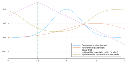
Consider for example a game on the real line where both and are Gaussian. Then the optimal Wasserstein critic and the optimal GAN discriminator are plotted as below:

For fixed discriminator, the generator needs to minimize the following objectives:
- For GAN, .
- For Wasserstein GAN, .
Let be parametrized by , then we can perform stochastic gradient descent by using two unbiased estimators of the gradient:where we used the reparametrization trick.[note 2]

As shown, the generator in GAN is motivated to let its "slide down the peak" of . Similarly for the generator in Wasserstein GAN.
For Wasserstein GAN, has gradient 1 almost everywhere, while for GAN, has flat gradient in the middle, and steep gradient elsewhere. As a result, the variance for the estimator in GAN is usually much larger than that in Wasserstein GAN. See also Figure 3 of.[1]
The problem with is much more severe in actual machine learning situations. Consider training a GAN to generate ImageNet, a collection of photos of size 256-by-256. The space of all such photos is , and the distribution of ImageNet pictures, , concentrates on a manifold of much lower dimension in it. Consequently, any generator strategy would almost surely be entirely disjoint from , making . Thus, a good discriminator can almost perfectly distinguish from , as well as any close to . Thus, the gradient , creating no learning signal for the generator.
Detailed theorems can be found in.[4]
Training Wasserstein GANs
Training the generator in Wasserstein GAN is just gradient descent, the same as in GAN (or most deep learning methods), but training the discriminator is different, as the discriminator is now restricted to have bounded Lipschitz norm. There are several methods for this.
Upper-bounding the Lipschitz norm
Let the discriminator function to be implemented by a multilayer perceptron:where , and is a fixed activation function with . For example, the hyperbolic tangent function satisfies the requirement.
Then, for any , let , we have by the chain rule:Thus, the Lipschitz norm of is upper-bounded bywhere is the operator norm of the matrix, that is, the largest singular value of the matrix, that is, the spectral radius of the matrix (these concepts are the same for matrices, but different for general linear operators).
Since , we have , and consequently the upper bound:Thus, if we can upper-bound operator norms of each matrix, we can upper-bound the Lipschitz norm of .
Weight clipping
Since for any matrix , let , we haveby clipping all entries of to within some interval , we have can bound .
This is the weight clipping method, proposed by the original paper.[1]
Spectral normalization
The spectral radius can be efficiently computed by the following algorithm:
INPUT matrix and initial guess
Iterate to convergence . This is the eigenvector of with eigenvalue .
RETURN
By reassigning after each update of the discriminator, we can upper bound , and thus upper bound .
The algorithm can be further accelerated by memoization: At step , store . Then at step , use as the initial guess for the algorithm. Since is very close to , so is close to , so this allows rapid convergence.
This is the spectral normalization method.[5]
Gradient penalty
Instead of strictly bounding , we can simply add a "gradient penalty" term for the discriminator, of formwhere is a fixed distribution used to estimate how much the discriminator has violated the Lipschitz norm requirement. The discriminator, in attempting to minimize the new loss function, would naturally bring close to everywhere, thus making .
This is the gradient penalty method.[6]
Further reading
- From GAN to WGAN
- Wasserstein GAN and the Kantorovich-Rubinstein Duality
- Depth First Learning: Wasserstein GAN
See also
References
- ↑ 1.0 1.1 1.2 Arjovsky, Martin; Chintala, Soumith; Bottou, Léon (2017-07-17). "Wasserstein Generative Adversarial Networks" (in en). International Conference on Machine Learning (PMLR): 214–223. https://proceedings.mlr.press/v70/arjovsky17a.html.
- ↑ Weng, Lilian (2019-04-18). "From GAN to WGAN". arXiv:1904.08994 [cs.LG].
- ↑ Nowozin, Sebastian; Cseke, Botond; Tomioka, Ryota (2016). "f-GAN: Training Generative Neural Samplers using Variational Divergence Minimization". Advances in Neural Information Processing Systems (Curran Associates, Inc.) 29. https://proceedings.neurips.cc/paper/2016/hash/cedebb6e872f539bef8c3f919874e9d7-Abstract.html.
- ↑ Arjovsky, Martin; Bottou, Léon (2017-01-01). Towards Principled Methods for Training Generative Adversarial Networks. https://ui.adsabs.harvard.edu/abs/2017arXiv170104862A.
- ↑ Miyato, Takeru; Kataoka, Toshiki; Koyama, Masanori; Yoshida, Yuichi (2018-02-16). "Spectral Normalization for Generative Adversarial Networks". arXiv:1802.05957 [cs.LG].
- ↑ Gulrajani, Ishaan; Ahmed, Faruk; Arjovsky, Martin; Dumoulin, Vincent; Courville, Aaron C (2017). "Improved Training of Wasserstein GANs". Advances in Neural Information Processing Systems (Curran Associates, Inc.) 30. https://proceedings.neurips.cc/paper/2017/hash/892c3b1c6dccd52936e27cbd0ff683d6-Abstract.html.
Notes
- ↑ In practice, the generator would never be able to reach perfect imitation, and so the discriminator would have motivation for perceiving the difference, which allows it to be used for other tasks, such as performing ImageNet classification without supervision.
- ↑ This is not how it is really done in practice, since is in general intractable, but it is theoretically illuminating.
 |

