Multilayer perceptron

Short description: Type of feedforward neural network

"MLP" is not to be confused with "NLP", which refers to natural language processing.

A multilayer perceptron (MLP) is a name for a modern feedforward artificial neural network, consisting of fully connected neurons with a nonlinear kind of activation function, organized in at least three layers, notable for being able to distinguish data that is not linearly separable. It is a misnomer because the original perceptron used a Heaviside step function, instead of a nonlinear kind of activation function (used by modern networks).

Modern feedforward networks are trained using the backpropagation method and are colloquially referred to as the "vanilla" neural networks.

Timeline

• In 1958, a layered network of perceptrons, consisting of an input layer, a hidden layer with randomized weights that did not learn, and an output layer with learning connections, was introduced already by Frank Rosenblatt in his book Perceptron. This extreme learning machine was not yet a deep learning network.

• In 1965, the first deep-learning feedforward network, not yet using stochastic gradient descent, was published by Alexey Grigorevich Ivakhnenko and Valentin Lapa, at the time called the Group Method of Data Handling.

• In 1967, a deep-learning network, which used stochastic gradient descent for the first time, able to classify non-linearily separable pattern classes, was published by Shun'ichi Amari. Amari's student Saito conducted the computer experiments, using a five-layered feedforward network with two learning layers.

• In 1970, modern backpropagation method, an efficient application of a chain-rule-based supervised learning, was for the first time published by the Finnish researcher Seppo Linnainmaa. The term (i.e. "back-propagating errors") itself has been used by Rosenblatt himself, but he did not know how to implement it, although a continuous precursor of backpropagation was already used in the context of control theory in 1960 by Henry J. Kelley. It is known also as a reverse mode of automatic differentiation.

• In 1982, backpropagation was applied in the way that has become standard, for the first time by Paul Werbos.

• In 1985, an experimental analysis of the technique was conducted by David E. Rumelhart et al.. Many improvements to the approach have been made in subsequent decades,.

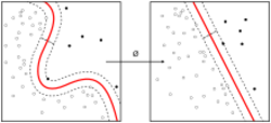
• In 1990s, an (much simpler) alternative to using neural networks, although still related support vector machine approach was developed by Vladimir Vapnik and his colleagues. In addition to performing linear classification, they were able to efficiently perform a non-linear classification using what is called the kernel trick, using high-dimensional feature spaces.

• In 2003, interest in backpropagation networks returned due to the successes of deep learning being applied to language modelling by Yoshua Bengio with co-authors.

• In 2017, modern transformer architectures has been introduced.

• In 2021, a very simple NN architecture combining two deep MLPs with skip connections and layer normalizations was designed and called MLP-Mixer; its realizations featuring 19 to 431 millions of parameters were shown to be comparable to vision transformers of similar size on ImageNet and similar image classification tasks.

Mathematical foundations

Activation function

If a multilayer perceptron has a linear activation function in all neurons, that is, a linear function that maps the weighted inputs to the output of each neuron, then linear algebra shows that any number of layers can be reduced to a two-layer input-output model. In MLPs some neurons use a nonlinear activation function that was developed to model the frequency of action potentials, or firing, of biological neurons.

The two historically common activation functions are both sigmoids, and are described by

[math]\displaystyle{ y(v_i) = \tanh(v_i) ~~ \textrm{and} ~~ y(v_i) = (1+e^{-v_i})^{-1} }[/math].

The first is a hyperbolic tangent that ranges from −1 to 1, while the other is the logistic function, which is similar in shape but ranges from 0 to 1. Here [math]\displaystyle{ y_i }[/math] is the output of the [math]\displaystyle{ i }[/math]th node (neuron) and [math]\displaystyle{ v_i }[/math] is the weighted sum of the input connections. Alternative activation functions have been proposed, including the rectifier and softplus functions. More specialized activation functions include radial basis functions (used in radial basis networks, another class of supervised neural network models).

In recent developments of deep learning the rectified linear unit (ReLU) is more frequently used as one of the possible ways to overcome the numerical problems related to the sigmoids.

Layers

The MLP consists of three or more layers (an input and an output layer with one or more hidden layers) of nonlinearly-activating nodes. Since MLPs are fully connected, each node in one layer connects with a certain weight [math]\displaystyle{ w_{ij} }[/math] to every node in the following layer.

Learning

Learning occurs in the perceptron by changing connection weights after each piece of data is processed, based on the amount of error in the output compared to the expected result. This is an example of supervised learning, and is carried out through backpropagation, a generalization of the least mean squares algorithm in the linear perceptron.

We can represent the degree of error in an output node [math]\displaystyle{ j }[/math] in the [math]\displaystyle{ n }[/math]th data point (training example) by [math]\displaystyle{ e_j(n)=d_j(n)-y_j(n) }[/math], where [math]\displaystyle{ d_j(n) }[/math] is the desired target value for [math]\displaystyle{ n }[/math]th data point at node [math]\displaystyle{ j }[/math], and [math]\displaystyle{ y_j(n) }[/math] is the value produced by the perceptron at node [math]\displaystyle{ j }[/math] when the [math]\displaystyle{ n }[/math]th data point is given as an input.

The node weights can then be adjusted based on corrections that minimize the error in the entire output for the [math]\displaystyle{ n }[/math]th data point, given by

[math]\displaystyle{ \mathcal{E}(n)=\frac{1}{2}\sum_{\text{output node }j} e_j^2(n) }[/math].

Using gradient descent, the change in each weight [math]\displaystyle{ w_{ij} }[/math] is

[math]\displaystyle{ \Delta w_{ji} (n) = -\eta\frac{\partial\mathcal{E}(n)}{\partial v_j(n)} y_i(n) }[/math]

where [math]\displaystyle{ y_i(n) }[/math] is the output of the previous neuron [math]\displaystyle{ i }[/math], and [math]\displaystyle{ \eta }[/math] is the learning rate, which is selected to ensure that the weights quickly converge to a response, without oscillations. In the previous expression, [math]\displaystyle{ \frac{\partial\mathcal{E}(n)}{\partial v_j(n)} }[/math] denotes the partial derivate of the error [math]\displaystyle{ \mathcal{E}(n) }[/math] according to the weighted sum [math]\displaystyle{ v_j(n) }[/math] of the input connections of neuron [math]\displaystyle{ i }[/math].

The derivative to be calculated depends on the induced local field [math]\displaystyle{ v_j }[/math], which itself varies. It is easy to prove that for an output node this derivative can be simplified to

[math]\displaystyle{ -\frac{\partial\mathcal{E}(n)}{\partial v_j(n)} = e_j(n)\phi^\prime (v_j(n)) }[/math]

where [math]\displaystyle{ \phi^\prime }[/math] is the derivative of the activation function described above, which itself does not vary. The analysis is more difficult for the change in weights to a hidden node, but it can be shown that the relevant derivative is

[math]\displaystyle{ -\frac{\partial\mathcal{E}(n)}{\partial v_j(n)} = \phi^\prime (v_j(n))\sum_k -\frac{\partial\mathcal{E}(n)}{\partial v_k(n)} w_{kj}(n) }[/math].

This depends on the change in weights of the [math]\displaystyle{ k }[/math]th nodes, which represent the output layer. So to change the hidden layer weights, the output layer weights change according to the derivative of the activation function, and so this algorithm represents a backpropagation of the activation function.

External links

• Weka: Open source data mining software with multilayer perceptron implementation.
• Neuroph Studio documentation, implements this algorithm and a few others.

de:Perzeptron#Mehrlagiges Perzeptron

References

- ↑ Cybenko, G. 1989. Approximation by superpositions of a sigmoidal function Mathematics of Control, Signals, and Systems, 2(4), 303–314.
- ↑ 2.0 2.1 Linnainmaa, Seppo (1970). The representation of the cumulative rounding error of an algorithm as a Taylor expansion of the local rounding errors (Masters) (in suomi). University of Helsinki. pp. 6–7.
- ↑ 3.0 3.1 Kelley, Henry J. (1960). "Gradient theory of optimal flight paths". ARS Journal 30 (10): 947–954. doi:10.2514/8.5282.
- ↑ Rosenblatt, Frank. x. Principles of Neurodynamics: Perceptrons and the Theory of Brain Mechanisms. Spartan Books, Washington DC, 1961
- ↑ 5.0 5.1 Werbos, Paul (1982). "Applications of advances in nonlinear sensitivity analysis". System modeling and optimization. Springer. pp. 762–770. http://werbos.com/Neural/SensitivityIFIPSeptember1981.pdf. Retrieved 2 July 2017.
- ↑ 6.0 6.1 Rumelhart, David E., Geoffrey E. Hinton, and R. J. Williams. "Learning Internal Representations by Error Propagation". David E. Rumelhart, James L. McClelland, and the PDP research group. (editors), Parallel distributed processing: Explorations in the microstructure of cognition, Volume 1: Foundation. MIT Press, 1986.
- ↑ Hastie, Trevor. Tibshirani, Robert. Friedman, Jerome. The Elements of Statistical Learning: Data Mining, Inference, and Prediction. Springer, New York, NY, 2009.
- ↑ Rosenblatt, Frank (1958). "The Perceptron: A Probabilistic Model For Information Storage And Organization in the Brain". Psychological Review 65 (6): 386–408. doi:10.1037/h0042519. PMID 13602029.
- ↑ 9.0 9.1 Rosenblatt, Frank (1962). Principles of Neurodynamics. Spartan, New York.
- ↑ 10.0 10.1 10.2 10.3 10.4 10.5 10.6 10.7 Schmidhuber, Juergen (2022). "Annotated History of Modern AI and Deep Learning". arXiv:2212.11279 [cs.NE].
- ↑ Huang, Guang-Bin; Zhu, Qin-Yu; Siew, Chee-Kheong (2006). "Extreme learning machine: theory and applications". Neurocomputing 70 (1): 489–501. doi:10.1016/j.neucom.2005.12.126.
- ↑ Ivakhnenko, A. G. (1973). Cybernetic Predicting Devices. CCM Information Corporation. https://books.google.com/books?id=FhwVNQAACAAJ.
- ↑ Ivakhnenko, A. G.; Grigorʹevich Lapa, Valentin (1967). Cybernetics and forecasting techniques. American Elsevier Pub. Co.. https://books.google.com/books?id=rGFgAAAAMAAJ.
- ↑ Amari, Shun'ichi (1967). "A theory of adaptive pattern classifier". IEEE Transactions EC (16): 279–307.
- ↑ Rodríguez, Omar Hernández; López Fernández, Jorge M. (2010). "A Semiotic Reflection on the Didactics of the Chain Rule". The Mathematics Enthusiast 7 (2): 321–332. doi:10.54870/1551-3440.1191. https://scholarworks.umt.edu/tme/vol7/iss2/10/. Retrieved 2019-08-04.
- ↑ Leibniz, Gottfried Wilhelm Freiherr von (1920) (in en). The Early Mathematical Manuscripts of Leibniz: Translated from the Latin Texts Published by Carl Immanuel Gerhardt with Critical and Historical Notes (Leibniz published the chain rule in a 1676 memoir). Open court publishing Company. ISBN 9780598818461. https://books.google.com/books?id=bOIGAAAAYAAJ&q=leibniz+altered+manuscripts&pg=PA90.
- ↑ Linnainmaa, Seppo (1976). "Taylor expansion of the accumulated rounding error". BIT Numerical Mathematics 16 (2): 146–160. doi:10.1007/bf01931367.
- ↑ R. Collobert and S. Bengio (2004). Links between Perceptrons, MLPs and SVMs. Proc. Int'l Conf. on Machine Learning (ICML).
- ↑ Bengio, Yoshua; Ducharme, Réjean; Vincent, Pascal; Janvin, Christian (March 2003). "A neural probabilistic language model". The Journal of Machine Learning Research 3: 1137–1155. https://dl.acm.org/doi/10.5555/944919.944966.
- ↑ Vaswani, Ashish; Shazeer, Noam; Parmar, Niki; Uszkoreit, Jakob; Jones, Llion; Gomez, Aidan N; Kaiser, Łukasz; Polosukhin, Illia (2017). "Attention is All you Need". Advances in Neural Information Processing Systems (Curran Associates, Inc.) 30. https://proceedings.neurips.cc/paper_files/paper/2017/hash/3f5ee243547dee91fbd053c1c4a845aa-Abstract.html.
- ↑ Geva, Mor; Schuster, Roei; Berant, Jonathan; Levy, Omer (2021). "Transformer Feed-Forward Layers Are Key-Value Memories". Proceedings of the 2021 Conference on Empirical Methods in Natural Language Processing. pp. 5484–5495. doi:10.18653/v1/2021.emnlp-main.446. https://aclanthology.org/2021.emnlp-main.446/.
- ↑ "Papers with Code – MLP-Mixer: An all-MLP Architecture for Vision". https://paperswithcode.com/paper/mlp-mixer-an-all-mlp-architecture-for-vision.
- ↑ Haykin, Simon (1998). Neural Networks: A Comprehensive Foundation (2 ed.). Prentice Hall. ISBN 0-13-273350-1.