Sequential quadratic programming

Short description: Optimization algorithm

Sequential quadratic programming (SQP) is an iterative method for constrained nonlinear optimization which may be considered a quasi-Newton method. SQP methods are used on mathematical problems for which the objective function and the constraints are twice continuously differentiable, but not necessarily convex.

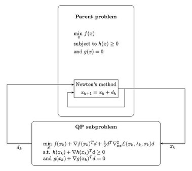
SQP methods solve a sequence of optimization subproblems, each of which optimizes a quadratic model of the objective subject to a linearization of the constraints. If the problem is unconstrained, then the method reduces to Newton's method for finding a point where the gradient of the objective vanishes. If the problem has only equality constraints, then the method is equivalent to applying Newton's method to the first-order optimality conditions, or Karush–Kuhn–Tucker conditions, of the problem.

Algorithm basics

Overview schematic illustrating the basic SQP algorithm

Consider a nonlinear programming problem of the form:

[math]\displaystyle{ \begin{array}{rl} \min\limits_{x} & f(x) \\ \mbox{subject to} & h(x) \ge 0 \\ & g(x) = 0. \end{array} }[/math]

The Lagrangian for this problem is

[math]\displaystyle{ \mathcal{L}(x,\lambda,\sigma) = f(x) - \lambda h(x) - \sigma g(x), }[/math]

where [math]\displaystyle{ \lambda }[/math] and [math]\displaystyle{ \sigma }[/math] are Lagrange multipliers.

The standard Newton's Method searches for the solution [math]\displaystyle{ \nabla \mathcal{L}(x,\lambda,\sigma) =0 }[/math] by iterating the following equation, where [math]\displaystyle{ \nabla^2_{xx} }[/math] denotes the Hessian matrix:

[math]\displaystyle{ \begin{bmatrix} x_{k+1} \\ \lambda_{k+1} \\ \sigma_{k+1} \end{bmatrix} = \begin{bmatrix} x_k \\ \lambda_k \\ \sigma_k \end{bmatrix} - \underbrace{ \begin{bmatrix} \nabla^2_{xx} \mathcal{L} & \nabla h & \nabla g \\ \nabla h^T & 0 & 0 \\ \nabla g^{T} & 0 & 0 \end{bmatrix}^{-1} }_{\nabla^2 \mathcal{L}} \underbrace{ \begin{bmatrix} \nabla f + \lambda_k \nabla h + \sigma_k \nabla g \\ h \\ g \end{bmatrix} }_{\nabla \mathcal{L}} }[/math].

However, because the matrix [math]\displaystyle{ \nabla^2 \mathcal{L} }[/math] is generally singular (and therefore non-invertible), the Newton step [math]\displaystyle{ d_k = \left( \nabla^2_{xx} \mathcal{L} \right)^{-1} \nabla \mathcal{L} }[/math] cannot be calculated directly. Instead the basic sequential quadratic programming algorithm defines an appropriate search direction [math]\displaystyle{ d_k }[/math] at an iterate [math]\displaystyle{ (x_k, \lambda_k, \sigma_k) }[/math], as a solution to the quadratic programming subproblem

[math]\displaystyle{ \begin{array}{rl} \min\limits_{d} & f(x_k) + \nabla f(x_k)^Td + \tfrac{1}{2} d^T \nabla^2_{xx} \mathcal{L}(x_k,\lambda_k,\sigma_k) d \\ \mathrm{s.t.} & h(x_k) + \nabla h(x_k)^Td \ge 0 \\ & g(x_k) + \nabla g(x_k)^T d = 0. \end{array} }[/math]

where the quadratic form is formed with the Hessian of the Lagrangian. Note that the term [math]\displaystyle{ f(x_k) }[/math] in the expression above may be left out for the minimization problem, since it is constant under the [math]\displaystyle{ \min\limits_{d} }[/math] operator.

Together, the SQP algorithm starts by first choosing the initial iterate [math]\displaystyle{ (x_0, \lambda_0, \sigma_0) }[/math], then calculating [math]\displaystyle{ \nabla^2 \mathcal{L}(x_0, \lambda_0, \sigma_0) }[/math] and [math]\displaystyle{ \nabla \mathcal{L}(x_0, \lambda_0, \sigma_0) }[/math]. Then the QP subproblem is built and solved to find the Newton step direction [math]\displaystyle{ d_0 }[/math] which is used to update the parent problem iterate using [math]\displaystyle{ \left[ x_{k+1}, \lambda_{k+1}, \sigma_{k+1} \right]^T = \left[ x_{k}, \lambda_{k}, \sigma_{k} \right]^T + d_k }[/math]. This process is repeated for [math]\displaystyle{ k = 0, 1, 2, \ldots }[/math] until the parent problem satisfies a convergence test.

Practical implementations

Practical implementations of the SQP algorithm are significantly more complex than its basic version above. To adapt SQP for real-world applications, the following challenges must be addressed:

• The possibility of an infeasible QP subproblem.
• QP subproblem yielding an bad step: one that either fails to reduce the target or increases constraints violation.
• Breakdown of iterations due to significant deviation of the target/constraints from their quadratic/linear models.

To overcome these challenges, various strategies are typically employed:

• Use of merit functions, which assess progress towards a constrained solution, or filter methods.
• Trust region or line search methods to manage deviations between the quadratic model and the actual target.
• Special feasibility restoration phases to handle infeasible subproblems, or the use of L1-penalized subproblems to gradually decrease infeasibility

These strategies can be combined in numerous ways, resulting in a diverse range of SQP methods.

Alternative approaches

• Sequential linear programming
• Sequential linear-quadratic programming
• Augmented Lagrangian method

Implementations

SQP methods have been implemented in well known numerical environments such as MATLAB and GNU Octave. There also exist numerous software libraries, including open source:

• SciPy (de facto standard for scientific Python) has scipy.optimize.minimize(method='SLSQP') solver.
• NLopt (C/C++ implementation, with numerous interfaces including Julia, Python, R, MATLAB/Octave), implemented by Dieter Kraft as part of a package for optimal control, and modified by S. G. Johnson.
• ALGLIB SQP solver (C++, C#, Java, Python API)

and commercial

• LabVIEW
• KNITRO (C, C++, C#, Java, Python, Julia, Fortran)
• NPSOL (Fortran)
• SNOPT (Fortran)
• NLPQL (Fortran)
• MATLAB
• SuanShu (Java)

See also

• Newton's method
• Secant method
• Model Predictive Control

References

• Bonnans, J. Frédéric; Gilbert, J. Charles; Lemaréchal, Claude; Sagastizábal, Claudia A. (2006). Numerical optimization: Theoretical and practical aspects. Universitext (Second revised ed. of translation of 1997 French ed.). Berlin: Springer-Verlag. pp. xiv+490. doi:10.1007/978-3-540-35447-5. ISBN 978-3-540-35445-1. https://www.springer.com/mathematics/applications/book/978-3-540-35445-1. 
• Jorge Nocedal and Stephen J. Wright (2006). Numerical Optimization. Springer.. ISBN 978-0-387-30303-1. http://www.ece.northwestern.edu/~nocedal/book/num-opt.html. 

External links

• Sequential Quadratic Programming at NEOS guide