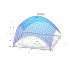
Nonlinear conjugate gradient method

Short description: Concept in mathematics

In numerical optimization, the nonlinear conjugate gradient method generalizes the conjugate gradient method to nonlinear optimization. For a quadratic function $f(x)$

$f(x)=\Vert Ax-b{\Vert }^2,$

the minimum of $f$ is obtained when the gradient is 0:

${\mathrm{\nabla }}_{x}f=2A^T(Ax-b)=0$.

Whereas linear conjugate gradient seeks a solution to the linear equation $A^{T}Ax=A^{T}b$, the nonlinear conjugate gradient method is generally used to find the local minimum of a nonlinear function using its gradient ${\mathrm{\nabla }}_{x}f$ alone. It works when the function is approximately quadratic near the minimum, which is the case when the function is twice differentiable at the minimum and the second derivative is non-singular there.

Given a function $f(x)$ of $N$ variables to minimize, its gradient ${\mathrm{\nabla }}_{x}f$ indicates the direction of maximum increase. One simply starts in the opposite (steepest descent) direction:

$\mathrm{\Delta }{x}_0=-{\mathrm{\nabla }}_{x}f(x_0)$

with an adjustable step length $\alpha$ and performs a line search in this direction until it reaches the minimum of $f$:

${\alpha }_0:=\arg \underset{\alpha }{\min }f(x_0+\alpha \mathrm{\Delta }{x}_0)$,

$x_1=x_0+{\alpha }_0\mathrm{\Delta }{x}_0$

After this first iteration in the steepest direction $\mathrm{\Delta }{x}_0$, the following steps constitute one iteration of moving along a subsequent conjugate direction $s_n$, where $s_0=\mathrm{\Delta }{x}_0$:

1. Calculate the steepest direction: $\mathrm{\Delta }{x}_n=-{\mathrm{\nabla }}_{x}f(x_n)$,
2. Compute ${\beta }_n$ according to one of the formulas below,
3. Update the conjugate direction: $s_n=\mathrm{\Delta }{x}_n+{\beta }_n{s}_{n-1}$
4. Perform a line search: optimize ${\alpha }_n=\arg \underset{\alpha }{\min }f(x_n+\alpha s_n)$,
5. Update the position: $x_{n+1}=x_n+{\alpha }_n{s}_n$,

With a pure quadratic function the minimum is reached within N iterations (excepting roundoff error), but a non-quadratic function will make slower progress. Subsequent search directions lose conjugacy requiring the search direction to be reset to the steepest descent direction at least every N iterations, or sooner if progress stops. However, resetting every iteration turns the method into steepest descent. The algorithm stops when it finds the minimum, determined when no progress is made after a direction reset (i.e. in the steepest descent direction), or when some tolerance criterion is reached.

Within a linear approximation, the parameters $\alpha$ and $\beta$ are the same as in the linear conjugate gradient method but have been obtained with line searches. The conjugate gradient method can follow narrow (ill-conditioned) valleys, where the steepest descent method slows down and follows a criss-cross pattern.

Four of the best known formulas for ${\beta }_n$ are named after their developers:

• Fletcher–Reeves:

${\beta }_n^{FR}=\frac{\mathrm{\Delta }{x}_n^T\mathrm{\Delta }{x}_n}{\mathrm{\Delta }{x}_{n-1}^T\mathrm{\Delta }{x}_{n-1}}.$

• Polak–Ribière:

${\beta }_n^{PR}=\frac{\mathrm{\Delta }{x}_n^T(\mathrm{\Delta }{x}_n-\mathrm{\Delta }{x}_{n-1})}{\mathrm{\Delta }{x}_{n-1}^T\mathrm{\Delta }{x}_{n-1}}.$

• Hestenes–Stiefel:

${\beta }_n^{HS}=\frac{\mathrm{\Delta }{x}_n^T(\mathrm{\Delta }{x}_n-\mathrm{\Delta }{x}_{n-1})}{-s_{n-1}^T(\mathrm{\Delta }{x}_n-\mathrm{\Delta }{x}_{n-1})}.$

• Dai–Yuan:

${\beta }_n^{DY}=\frac{\mathrm{\Delta }{x}_n^T\mathrm{\Delta }{x}_n}{-s_{n-1}^T(\mathrm{\Delta }{x}_n-\mathrm{\Delta }{x}_{n-1})}.$.

These formulas are equivalent for a quadratic function, but for nonlinear optimization the preferred formula is a matter of heuristics or taste. A popular choice is $\beta =\max \{0,{\beta }^{PR}\}$, which provides a direction reset automatically.

Algorithms based on Newton's method potentially converge much faster. There, both step direction and length are computed from the gradient as the solution of a linear system of equations, with the coefficient matrix being the exact Hessian matrix (for Newton's method proper) or an estimate thereof (in the quasi-Newton methods, where the observed change in the gradient during the iterations is used to update the Hessian estimate). For high-dimensional problems, the exact computation of the Hessian is usually prohibitively expensive, and even its storage can be problematic, requiring $O(N^2)$ memory (but see the limited-memory L-BFGS quasi-Newton method).

The conjugate gradient method can also be derived using optimal control theory. In this accelerated optimization theory, the conjugate gradient method falls out as a nonlinear optimal feedback controller,

$u=k(x,\dot{x}):=-{\gamma }_a{\mathrm{\nabla }}_{x}f(x)-{\gamma }_b\dot{x}$

for the double integrator system,

$\ddot{x}=u$

The quantities ${\gamma }_a>0$ and ${\gamma }_b>0$ are variable feedback gains.

See also

• Gradient descent
• Broyden–Fletcher–Goldfarb–Shanno algorithm
• Conjugate gradient method
• L-BFGS (limited memory BFGS)
• Nelder–Mead method
• Wolfe conditions

References

- ↑ Fletcher, R.; Reeves, C. M. (1964). "Function minimization by conjugate gradients". The Computer Journal 7 (2): 149–154. doi:10.1093/comjnl/7.2.149.
- ↑ Polak, E.; Ribière, G. (1969). "Note sur la convergence de méthodes de directions conjuguées". Revue Française d'Automatique, Informatique, Recherche Opérationnelle 3 (1): 35–43.
- ↑ Hestenes, M. R.; Stiefel, E. (1952). "Methods of Conjugate Gradients for Solving Linear Systems". Journal of Research of the National Bureau of Standards 49 (6): 409–436. doi:10.6028/jres.049.044.
- ↑ Dai, Y.-H.; Yuan, Y. (1999). "A nonlinear conjugate gradient method with a strong global convergence property". SIAM Journal on Optimization 10 (1): 177–182. doi:10.1137/S1052623497318992.
- ↑ Shewchuk, J. R. (August 1994). "An Introduction to the Conjugate Gradient Method Without the Agonizing Pain". https://www.cs.cmu.edu/~quake-papers/painless-conjugate-gradient.pdf.
- ↑ 6.0 6.1 Ross, I. M. (2019). "An Optimal Control Theory for Accelerated Optimization". arXiv:1902.09004 [math.OC].