Weak supervision

Short description: A paradigm in machine learning

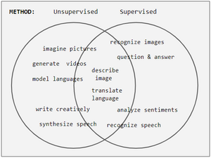
Weak supervision is a paradigm in machine learning, the relevance and notability of which increased with the advent of large language models due to large amount of data required to train them. It is characterized by using a combination of a small amount of human-labeled data (exclusively used in more expensive and time-consuming supervised learning paradigm), followed by a large amount of unlabeled data (used exclusively in unsupervised learning paradigm). In other words, the desired output values are provided only for a subset of the training data. The remaining data is unlabeled or imprecisely labeled. Intuitively, it can be seen as an exam and labeled data as sample problems that the teacher solves for the class as an aid in solving another set of problems. In the transductive setting, these unsolved problems act as exam questions. In the inductive setting, they become practice problems of the sort that will make up the exam. Technically, it could be viewed as performing clustering and then labeling the clusters with the labeled data, pushing the decision boundary away from high-density regions, or learning an underlying one-dimensional manifold where the data reside.

Problem

Tendency for a task to employ supervised vs. unsupervised methods. Task names straddling circle boundaries is intentional. It shows that the classical division of imaginative tasks (left) employing unsupervised methods is blurred in today's learning schemes.

The acquisition of labeled data for a learning problem often requires a skilled human agent (e.g. to transcribe an audio segment) or a physical experiment (e.g. determining the 3D structure of a protein or determining whether there is oil at a particular location). The cost associated with the labeling process thus may render large, fully labeled training sets infeasible, whereas acquisition of unlabeled data is relatively inexpensive. In such situations, semi-supervised learning can be of great practical value. Semi-supervised learning is also of theoretical interest in machine learning and as a model for human learning.

Technique

An example of the influence of unlabeled data in semi-supervised learning. The top panel shows a decision boundary we might adopt after seeing only one positive (white circle) and one negative (black circle) example. The bottom panel shows a decision boundary we might adopt if, in addition to the two labeled examples, we were given a collection of unlabeled data (gray circles).

More formally, semi-supervised learning assumes a set of [math]\displaystyle{ l }[/math] independently identically distributed examples [math]\displaystyle{ x_1,\dots,x_l \in X }[/math] with corresponding labels [math]\displaystyle{ y_1,\dots,y_l \in Y }[/math] and [math]\displaystyle{ u }[/math] unlabeled examples [math]\displaystyle{ x_{l+1},\dots,x_{l+u} \in X }[/math] are processed. Semi-supervised learning combines this information to surpass the classification performance that can be obtained either by discarding the unlabeled data and doing supervised learning or by discarding the labels and doing unsupervised learning.

Semi-supervised learning may refer to either transductive learning or inductive learning. The goal of transductive learning is to infer the correct labels for the given unlabeled data [math]\displaystyle{ x_{l+1},\dots,x_{l+u} }[/math] only. The goal of inductive learning is to infer the correct mapping from [math]\displaystyle{ X }[/math] to [math]\displaystyle{ Y }[/math].

It is unnecessary (and, according to Vapnik's principle, imprudent) to perform transductive learning by way of inferring a classification rule over the entire input space; however, in practice, algorithms formally designed for transduction or induction are often used interchangeably.

Assumptions

In order to make any use of unlabeled data, some relationship to the underlying distribution of data must exist. Semi-supervised learning algorithms make use of at least one of the following assumptions:

Continuity / smoothness assumption

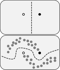
Points that are close to each other are more likely to share a label. This is also generally assumed in supervised learning and yields a preference for geometrically simple decision boundaries. In the case of semi-supervised learning, the smoothness assumption additionally yields a preference for decision boundaries in low-density regions, so few points are close to each other but in different classes.

Cluster assumption

The data tend to form discrete clusters, and points in the same cluster are more likely to share a label (although data that shares a label may spread across multiple clusters). This is a special case of the smoothness assumption and gives rise to feature learning with clustering algorithms.

Manifold assumption

The data lie approximately on a manifold of much lower dimension than the input space. In this case learning the manifold using both the labeled and unlabeled data can avoid the curse of dimensionality. Then learning can proceed using distances and densities defined on the manifold.

The manifold assumption is practical when high-dimensional data are generated by some process that may be hard to model directly, but which has only a few degrees of freedom. For instance, human voice is controlled by a few vocal folds, and images of various facial expressions are controlled by a few muscles. In these cases, it is better to consider distances and smoothness in the natural space of the generating problem, rather than in the space of all possible acoustic waves or images, respectively.

History

The heuristic approach of self-training (also known as self-learning or self-labeling) is historically the oldest approach to semi-supervised learning, with examples of applications starting in the 1960s.

The transductive learning framework was formally introduced by Vladimir Vapnik in the 1970s. Interest in inductive learning using generative models also began in the 1970s. A probably approximately correct learning bound for semi-supervised learning of a Gaussian mixture was demonstrated by Ratsaby and Venkatesh in 1995.

Methods

Generative models

Generative approaches to statistical learning first seek to estimate [math]\displaystyle{ p(x|y) }[/math], the distribution of data points belonging to each class. The probability [math]\displaystyle{ p(y|x) }[/math] that a given point [math]\displaystyle{ x }[/math] has label [math]\displaystyle{ y }[/math] is then proportional to [math]\displaystyle{ p(x|y)p(y) }[/math] by Bayes' rule. Semi-supervised learning with generative models can be viewed either as an extension of supervised learning (classification plus information about [math]\displaystyle{ p(x) }[/math]) or as an extension of unsupervised learning (clustering plus some labels).

Generative models assume that the distributions take some particular form [math]\displaystyle{ p(x|y,\theta) }[/math] parameterized by the vector [math]\displaystyle{ \theta }[/math]. If these assumptions are incorrect, the unlabeled data may actually decrease the accuracy of the solution relative to what would have been obtained from labeled data alone. However, if the assumptions are correct, then the unlabeled data necessarily improves performance.

The unlabeled data are distributed according to a mixture of individual-class distributions. In order to learn the mixture distribution from the unlabeled data, it must be identifiable, that is, different parameters must yield different summed distributions. Gaussian mixture distributions are identifiable and commonly used for generative models.

The parameterized joint distribution can be written as [math]\displaystyle{ p(x,y|\theta)=p(y|\theta)p(x|y,\theta) }[/math] by using the chain rule. Each parameter vector [math]\displaystyle{ \theta }[/math] is associated with a decision function [math]\displaystyle{ f_\theta(x) = \underset{y}{\operatorname{argmax}}\ p(y|x,\theta) }[/math]. The parameter is then chosen based on fit to both the labeled and unlabeled data, weighted by [math]\displaystyle{ \lambda }[/math]:

[math]\displaystyle{ \underset{\Theta}{\operatorname{argmax}}\left( \log p(\{x_i,y_i\}_{i=1}^l | \theta) + \lambda \log p(\{x_i\}_{i=l+1}^{l+u}|\theta)\right) }[/math]

Low-density separation

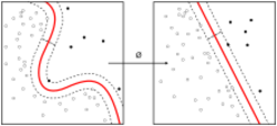
Another major class of methods attempts to place boundaries in regions with few data points (labeled or unlabeled). One of the most commonly used algorithms is the transductive support vector machine, or TSVM (which, despite its name, may be used for inductive learning as well). Whereas support vector machines for supervised learning seek a decision boundary with maximal margin over the labeled data, the goal of TSVM is a labeling of the unlabeled data such that the decision boundary has maximal margin over all of the data. In addition to the standard hinge loss [math]\displaystyle{ (1-yf(x))_+ }[/math] for labeled data, a loss function [math]\displaystyle{ (1-|f(x)|)_+ }[/math] is introduced over the unlabeled data by letting [math]\displaystyle{ y=\operatorname{sign}{f(x)} }[/math]. TSVM then selects [math]\displaystyle{ f^*(x) = h^*(x) + b }[/math] from a reproducing kernel Hilbert space [math]\displaystyle{ \mathcal{H} }[/math] by minimizing the regularized empirical risk:

[math]\displaystyle{ f^* = \underset{f}{\operatorname{argmin}}\left( \displaystyle \sum_{i=1}^l(1-y_if(x_i))_+ + \lambda_1 \|h\|_\mathcal{H}^2 + \lambda_2 \sum_{i=l+1}^{l+u} (1-|f(x_i)|)_+ \right) }[/math]

An exact solution is intractable due to the non-convex term [math]\displaystyle{ (1-|f(x)|)_+ }[/math], so research focuses on useful approximations.

Other approaches that implement low-density separation include Gaussian process models, information regularization, and entropy minimization (of which TSVM is a special case).

Laplacian regularization

Laplacian regularization has been historically approached through graph-Laplacian. Graph-based methods for semi-supervised learning use a graph representation of the data, with a node for each labeled and unlabeled example. The graph may be constructed using domain knowledge or similarity of examples; two common methods are to connect each data point to its [math]\displaystyle{ k }[/math] nearest neighbors or to examples within some distance [math]\displaystyle{ \epsilon }[/math]. The weight [math]\displaystyle{ W_{ij} }[/math] of an edge between [math]\displaystyle{ x_i }[/math] and [math]\displaystyle{ x_j }[/math] is then set to [math]\displaystyle{ e^{-\|x_i-x_j\|^2 / \epsilon^2} }[/math].

Within the framework of manifold regularization, the graph serves as a proxy for the manifold. A term is added to the standard Tikhonov regularization problem to enforce smoothness of the solution relative to the manifold (in the intrinsic space of the problem) as well as relative to the ambient input space. The minimization problem becomes

[math]\displaystyle{ \underset{f\in\mathcal{H}}{\operatorname{argmin}}\left( \frac{1}{l}\displaystyle\sum_{i=1}^l V(f(x_i),y_i) + \lambda_A \|f\|^2_\mathcal{H} + \lambda_I \int_\mathcal{M}\|\nabla_\mathcal{M} f(x)\|^2dp(x) \right) }[/math]

where [math]\displaystyle{ \mathcal{H} }[/math] is a reproducing kernel Hilbert space and [math]\displaystyle{ \mathcal{M} }[/math] is the manifold on which the data lie. The regularization parameters [math]\displaystyle{ \lambda_A }[/math] and [math]\displaystyle{ \lambda_I }[/math] control smoothness in the ambient and intrinsic spaces respectively. The graph is used to approximate the intrinsic regularization term. Defining the graph Laplacian [math]\displaystyle{ L = D - W }[/math] where [math]\displaystyle{ D_{ii} = \sum_{j=1}^{l+u} W_{ij} }[/math] and [math]\displaystyle{ \mathbf{f} }[/math] is the vector [math]\displaystyle{ [f(x_1)\dots f(x_{l+u})] }[/math], we have

[math]\displaystyle{ \mathbf{f}^T L \mathbf{f} = \displaystyle\sum_{i,j=1}^{l+u}W_{ij}(f_i-f_j)^2 \approx \int_\mathcal{M}\|\nabla_\mathcal{M} f(x)\|^2dp(x) }[/math].

The graph-based approach to Laplacian regularization is to put in relation with finite difference method.

The Laplacian can also be used to extend the supervised learning algorithms: regularized least squares and support vector machines (SVM) to semi-supervised versions Laplacian regularized least squares and Laplacian SVM.

Heuristic approaches

Some methods for semi-supervised learning are not intrinsically geared to learning from both unlabeled and labeled data, but instead make use of unlabeled data within a supervised learning framework. For instance, the labeled and unlabeled examples [math]\displaystyle{ x_1,\dots,x_{l+u} }[/math] may inform a choice of representation, distance metric, or kernel for the data in an unsupervised first step. Then supervised learning proceeds from only the labeled examples. In this vein, some methods learn a low-dimensional representation using the supervised data and then apply either low-density separation or graph-based methods to the learned representation. Iteratively refining the representation and then performing semi-supervised learning on said representation may further improve performance.

Self-training is a wrapper method for semi-supervised learning. First a supervised learning algorithm is trained based on the labeled data only. This classifier is then applied to the unlabeled data to generate more labeled examples as input for the supervised learning algorithm. Generally only the labels the classifier is most confident in are added at each step. In natural language processing, a common self-training algorithm is the Yarowsky algorithm for problems like word sense disambiguation, accent restoration, and spelling correction.

Co-training is an extension of self-training in which multiple classifiers are trained on different (ideally disjoint) sets of features and generate labeled examples for one another.

In human cognition

Human responses to formal semi-supervised learning problems have yielded varying conclusions about the degree of influence of the unlabeled data. More natural learning problems may also be viewed as instances of semi-supervised learning. Much of human concept learning involves a small amount of direct instruction (e.g. parental labeling of objects during childhood) combined with large amounts of unlabeled experience (e.g. observation of objects without naming or counting them, or at least without feedback).

Human infants are sensitive to the structure of unlabeled natural categories such as images of dogs and cats or male and female faces. Infants and children take into account not only unlabeled examples, but the sampling process from which labeled examples arise.

See also

• PU learning

Sources

• Chapelle, Olivier; Schölkopf, Bernhard; Zien, Alexander (2006). Semi-supervised learning. Cambridge, Mass.: MIT Press. ISBN 978-0-262-03358-9. 

External links

• Manifold Regularization A freely available MATLAB implementation of the graph-based semi-supervised algorithms Laplacian support vector machines and Laplacian regularized least squares.
• KEEL: A software tool to assess evolutionary algorithms for Data Mining problems (regression, classification, clustering, pattern mining and so on) KEEL module for semi-supervised learning.
• Semi-Supervised Learning Software
• Semi-Supervised learning — scikit-learn documentation Semi-supervised learning in scikit-learn.

References

- ↑ Semi-Supervised Learning Literature Survey, Page 5, 2007
- ↑ 2.0 2.1 Chapelle, Schölkopf & Zien 2006.
- ↑ Chawla, N., Bowyer, K., Hall, L.O., & Kegelmeyer, W.P. (2002). SMOTE: Synthetic Minority Over-sampling Technique. ArXiv, abs/1106.1813.
- ↑ Stevens, Kenneth N. (1998). Acoustic phonetics. Cambridge, Mass.: MIT Press. ISBN 0-585-08720-2. OCLC 42856189.
- ↑ Scudder, H. (July 1965). "Probability of error of some adaptive pattern-recognition machines". IEEE Transactions on Information Theory 11 (3): 363–371. doi:10.1109/TIT.1965.1053799. ISSN 1557-9654.
- ↑ Vapnik, V.; Chervonenkis, A. (1974) (in ru). Theory of Pattern Recognition. Moscow: Nauka. cited in Chapelle, Schölkopf & Zien 2006, p. 3
- ↑ 7.0 7.1 Ratsaby, J.; Venkatesh, S.. "Learning from a mixture of labeled and unlabeled examples with parametric side information". http://www.ariel.ac.il/sites/ratsaby/Publications/PDF/colt95.pdf. in Proceedings of the eighth annual conference on Computational learning theory - COLT '95. New York, New York, US: ACM Press. 1995. pp. 412–417. doi:10.1145/225298.225348. ISBN 0-89791-723-5.. Cited in Chapelle, Schölkopf & Zien 2006, p. 4
- ↑ Fabio, Cozman; Ira, Cohen (2006-09-22), "Risks of Semi-Supervised Learning: How Unlabeled Data Can Degrade Performance of Generative Classifiers", Semi-Supervised Learning (The MIT Press): pp. 56–72, doi:10.7551/mitpress/9780262033589.003.0004, ISBN 978-0-262-03358-9 In: Chapelle, Schölkopf & Zien 2006
- ↑ 9.0 9.1 9.2 Zhu, Xiaojin. Semi-Supervised Learning University of Wisconsin-Madison.
- ↑ M. Belkin; P. Niyogi (2004). "Semi-supervised Learning on Riemannian Manifolds". Machine Learning 56 (Special Issue on Clustering): 209–239. doi:10.1023/b:mach.0000033120.25363.1e. http://booksc.org/dl/11288633/421f61.
- ↑ M. Belkin, P. Niyogi, V. Sindhwani. On Manifold Regularization. AISTATS 2005.
- ↑ Iscen, Ahmet; Tolias, Giorgos; Avrithis, Yannis; Chum, Ondrej (2019). "Label Propagation for Deep Semi-Supervised Learning". 2019 IEEE/CVF Conference on Computer Vision and Pattern Recognition (CVPR). pp. 5065–5074. doi:10.1109/CVPR.2019.00521. ISBN 978-1-7281-3293-8.
- ↑ Burkhart, Michael C.; Shan, Kyle (2020). "Deep Low-Density Separation for Semi-supervised Classification". International Conference on Computational Science (ICCS). Lecture Notes in Computer Science. 12139. pp. 297–311. doi:10.1007/978-3-030-50420-5_22. ISBN 978-3-030-50419-9.
- ↑ Triguero, Isaac; García, Salvador; Herrera, Francisco (2013-11-26). "Self-labeled techniques for semi-supervised learning: taxonomy, software and empirical study" (in en). Knowledge and Information Systems 42 (2): 245–284. doi:10.1007/s10115-013-0706-y. ISSN 0219-1377.
- ↑ Fazakis, Nikos; Karlos, Stamatis; Kotsiantis, Sotiris; Sgarbas, Kyriakos (2015-12-29). "Self-Trained LMT for Semisupervised Learning" (in en). Computational Intelligence and Neuroscience 2016. doi:10.1155/2016/3057481. PMID 26839531.
- ↑ Yarowsky, David (1995). "Unsupervised Word Sense Disambiguation Rivaling Supervised Methods". Proceedings of the 33rd Annual Meeting of the Association for Computational Linguistics (Cambridge, MA: Association for Computational Linguistics): 189–196. doi:10.3115/981658.981684. https://aclanthology.org/P95-1026/. Retrieved 1 November 2022.
- ↑ Didaci, Luca; Fumera, Giorgio; Roli, Fabio (2012-11-07). Gimel'farb, Georgy. ed (in en). Analysis of Co-training Algorithm with Very Small Training Sets. Lecture Notes in Computer Science. Springer Berlin Heidelberg. pp. 719–726. doi:10.1007/978-3-642-34166-3_79. ISBN 978-3-642-34165-6.
- ↑ Zhu, Xiaojin (2009). Introduction to semi-supervised learning. Goldberg, A. B. (Andrew B.). [San Rafael, Calif.]: Morgan & Claypool Publishers. ISBN 978-1-59829-548-1. OCLC 428541480.
- ↑ Younger B. A.; Fearing D. D. (1999). "Parsing Items into Separate Categories: Developmental Change in Infant Categorization". Child Development 70 (2): 291–303. doi:10.1111/1467-8624.00022.
- ↑ Xu, F.; Tenenbaum, J. B. (2007). "Sensitivity to sampling in Bayesian word learning". Developmental Science 10 (3): 288–297. doi:10.1111/j.1467-7687.2007.00590.x. PMID 17444970.
- ↑ Gweon, H., Tenenbaum J.B., and Schulz L.E (2010). "Infants consider both the sample and the sampling process in inductive generalization". Proc Natl Acad Sci U S A 107 (20): 9066–71. doi:10.1073/pnas.1003095107. PMID 20435914. Bibcode: 2010PNAS..107.9066G.
- ↑ Martínez-Heredia, Antonio M.; Ventura, Sebastián (2025). "Weak Supervision: A Survey on Predictive Maintenance" (in en). WIREs Data Mining and Knowledge Discovery 15 (2). doi:10.1002/widm.70022. ISSN 1942-4787. https://wires.onlinelibrary.wiley.com/doi/10.1002/widm.70022.