Exponential function: Difference between revisions
over-write |
add |
||
| Line 1: | Line 1: | ||
{{Short description|Mathematical function, denoted exp(x) or e^x}} | {{Short description|Mathematical function, denoted exp(x) or e^x}} | ||
{{Infobox mathematical function | {{Infobox mathematical function | ||
| name = Exponential | | name = Exponential | ||
| Line 17: | Line 16: | ||
| reciprocal = <math>\exp(-z)</math> | | reciprocal = <math>\exp(-z)</math> | ||
| inverse = [[Natural logarithm]], [[Complex logarithm]] | | inverse = [[Natural logarithm]], [[Complex logarithm]] | ||
| derivative = <math>\ | | derivative = <math>\frac{\mathrm{d}}{\mathrm{d}\!\,z} \exp z = \exp z</math> | ||
| antiderivative = <math>\int \exp z\,dz = \exp z + C</math> | | antiderivative = <math>\int \exp z\,dz = \exp z + C</math> | ||
| taylor_series = <math>\exp z = \sum_{n=0}^\infty\frac{z^n}{n!}</math> | | taylor_series = <math>\exp z = \sum_{n=0}^\infty\frac{z^n}{n!}</math> | ||
}} | }} | ||
In [[Mathematics|mathematics]], the '''exponential function''' is the unique [[Real function|real function]] which maps [[0|zero]] to [[1|one]] and has a [[Derivative|derivative]] everywhere equal to its value. | In [[Mathematics|mathematics]], the '''exponential function''' is the unique [[Real function|real function]] which maps [[0|zero]] to [[1|one]] and has a [[Derivative|derivative]] everywhere equal to its value. It is denoted {{tmath|e^x}} or {{tmath|\exp x}}; the latter is preferred when the argument {{tmath|x}} is a complicated expression.<ref>{{cite web |title=Reviews of Modern Physics Style Guide |url=https://cdn.journals.aps.org/files/rmpguide.pdf |publisher=American Physical Society |access-date=30 December 2025 |location=XVI.B.1(d) |page=18 |quote=Which form to use, {{tmath|e}} or {{tmath|\exp}}, is determined by the number of characters and the complexity of the argument. The {{tmath|e}} form is appropriate when the argument is short and simple, i.e., <math>e^{i \mathbf{k}\cdot\mathbf{r}}</math>, whereas {{tmath|\exp}} should be used if the argument is more complicated.}}</ref><ref>{{cite book |author1=T. W. Chaundy |author2=P. R. Barrett |author3=Charles Batey |title=The Printing of Mathematics |date=1954 |publisher=Oxford University Press |page=31 |url=https://archive.org/details/printingofmathem0000chau/page/31/}}</ref> It is called ''exponential'' because its argument can be seen as an exponent to which a constant [[e (mathematical constant)|number {{math|''e'' ≈ 2.718}}]], the base, is raised. There are several other definitions of the exponential function, which are all equivalent although being of very different nature. | ||
The exponential function converts sums to products: | The exponential function converts sums to products: {{tmath|1=\exp(x + y) = \exp x \cdot \exp y }}. Its [[Inverse function|inverse function]], the [[Natural logarithm|natural logarithm]], {{tmath|\ln}} or {{tmath|\log}}, converts products to sums: {{tmath|1= \ln(x\cdot y) = \ln x + \ln y}}. | ||
The exponential function is occasionally called the '''natural exponential function''', matching the name ''natural logarithm'', for distinguishing it from some other functions that are also commonly called ''exponential functions''. These functions include the functions of the form {{tmath|1=f(x) = b^x}}, which is [[Exponentiation|exponentiation]] with a fixed base {{tmath|b}}. More generally, and especially in applications, functions of the general form {{tmath|1=f(x) = ab^x}} are also called exponential functions. They [[Exponential growth|grow]] or [[Exponential decay|decay]] exponentially in that the rate that {{tmath|f(x)}} changes when {{tmath|x}} is increased is ''proportional'' to the current value of {{tmath|f(x)}}. | The exponential function is occasionally called the '''natural exponential function''', matching the name ''natural logarithm'', for distinguishing it from some other functions that are also commonly called ''exponential functions''. These functions include the functions of the form {{tmath|1=f(x) = b^x}}, which is [[Exponentiation|exponentiation]] with a fixed base {{tmath|b}}. More generally, and especially in applications, functions of the general form {{tmath|1=f(x) = ab^x}} are also called exponential functions. They [[Exponential growth|grow]] or [[Exponential decay|decay]] exponentially in that the rate that {{tmath|f(x)}} changes when {{tmath|x}} is increased is ''proportional'' to the current value of {{tmath|f(x)}}. | ||
The exponential function can be generalized to accept [[Complex number|complex number]]s as arguments. This reveals relations between multiplication of complex numbers, rotations in the [[Complex plane|complex plane]], and [[Trigonometry|trigonometry]]. [[Euler's formula]] {{tmath|1= | The exponential function can be generalized to accept [[Complex number|complex number]]s as arguments. This reveals relations between multiplication of complex numbers, rotations in the [[Complex plane|complex plane]], and [[Trigonometry|trigonometry]]. [[Euler's formula]] {{tmath|1= e^{i\theta} = \cos\theta + i\sin\theta}} expresses and summarizes these relations. | ||
The exponential function can be even further generalized to accept other types of arguments, such as matrices and elements of [[Exponential map (Lie theory)|Lie algebras]]. | The exponential function can be even further generalized to accept other types of arguments, such as matrices and elements of [[Exponential map (Lie theory)|Lie algebras]]. | ||
| Line 42: | Line 41: | ||
[[Image:Exp tangent.svg|thumb|right |The derivative of the exponential function is equal to the value of the function. Since the derivative is the [[Slope|slope]] of the tangent, this implies that all green [[Right triangle|right triangle]]s have a base length of 1.]] | [[Image:Exp tangent.svg|thumb|right |The derivative of the exponential function is equal to the value of the function. Since the derivative is the [[Slope|slope]] of the tangent, this implies that all green [[Right triangle|right triangle]]s have a base length of 1.]] | ||
The exponential function is the unique [[Differentiable function|differentiable function]] that equals its [[Derivative|derivative]], and takes the value {{math|1}} for the value {{math|0}} of its variable. | |||
This | This definition requires a uniqueness proof and an existence proof, but it allows an easy derivation of the main properties of the exponential function. | ||
===Inverse of natural logarithm=== | ===Inverse of natural logarithm=== | ||
The exponential function is the [[Inverse function|inverse function]] of the [[Natural logarithm|natural logarithm]]. That is, | |||
:<math>\begin{align} | :<math>\begin{align} | ||
\ln (\exp x)&=x\\ | \ln (\exp x)&=x\\ | ||
| Line 59: | Line 54: | ||
===Power series=== | ===Power series=== | ||
The exponential function is the sum of the [[Power series|power series]]<ref name="Rudin_1987"/><ref name=":0">{{Cite web|last=Weisstein| first=Eric W.|title=Exponential Function|url=https://mathworld.wolfram.com/ExponentialFunction.html|access-date=2020-08-28| website=mathworld.wolfram.com|language=en}}</ref> | |||
<math display=block> | <math display=block> | ||
\begin{align}\exp(x) &= 1+x+\frac{x^2}{2!}+ \frac{x^3}{3!}+\cdots\\ | \begin{align}\exp(x) &= 1+x+\frac{x^2}{2!}+ \frac{x^3}{3!}+\cdots\\ | ||
&=\sum_{n=0}^\infty \frac{x^n}{n!},\end{align}</math> | &=\sum_{n=0}^\infty \frac{x^n}{n!},\end{align}</math> | ||
[[Image:Exp series.gif|right|thumb|The exponential function (in blue), and the sum of the first {{math|''n'' + 1}} terms of its power series (in red)]] | [[Image:Exp series.gif|right|thumb|The exponential function (in blue), and the sum of the first {{math|''n'' + 1}} terms of its power series (in red)]] | ||
where <math>n!</math> is the [[Factorial|factorial]] of {{mvar|n}} (the product of the {{mvar|n}} first positive integers). This series is absolutely convergent for every <math>x</math> | where <math>n!</math> is the [[Factorial|factorial]] of {{mvar|n}} (the product of the {{mvar|n}} first positive integers). This series is absolutely convergent for every <math>x</math>, by the [[Ratio test|ratio test]]. This shows that the exponential function is defined for every {{tmath|x}}, and is everywhere the sum of its [[Maclaurin series]]. | ||
===Functional equation=== | ===Functional equation=== | ||
The exponential satisfies the [[Functional equation|functional equation]] | |||
<math display=block>\exp(x+y)= \exp(x)\cdot \exp(y) | <math display=block>\exp(x+y)= \exp(x)\cdot \exp(y)</math> | ||
and maps the [[Additive identity|additive identity]] {{math|0}} to the multiplicative identity {{math|1}}. | |||
<math> f(x)= | The same equation is satisfied by other continuous functions <math>f(x)=b^x</math> that exponentiate their argument with an arbitrary base <math>b</math>.<ref>{{cite book | ||
| last = Jung | first = Soon-Mo | |||
| contribution = Chapter 9: Exponential Functional Equations | |||
| doi = 10.1007/978-1-4419-9637-4_9 | |||
| isbn = 9781441996374 | |||
| series = Springer Optimization and Its Applications | |||
| pages = 207–225 | |||
| publisher = Springer New York | |||
| title = Hyers-Ulam-Rassias Stability of Functional Equations in Nonlinear Analysis | |||
| year = 2011 | |||
| volume = 48 | |||
}}</ref> Among these functions, the exponential function is characterized by the property that its derivative at {{math|0}} is {{math|1}}.<ref>{{cite book | |||
| last1 = Aczél | first1 = J. | |||
| last2 = Dhombres | first2 = J. | |||
| doi = 10.1017/CBO9781139086578 | |||
| isbn = 0-521-35276-2 | |||
| mr = 1004465 | |||
| page = 10 | |||
| publisher = Cambridge University Press, Cambridge | |||
| series = Encyclopedia of Mathematics and its Applications | |||
| title = Functional Equations in Several Variables | |||
| volume = 31 | |||
| year = 1989}}</ref> | |||
===Limit of integer powers=== | ===Limit of integer powers=== | ||
The exponential function is the [[Limit (mathematics)|limit]], as the integer {{mvar|n}} goes to infinity,<ref name="Maor"/><ref name=":0" /> | |||
<math display=block>\exp(x)=\lim_{n \to +\infty} \left(1+\frac xn\right)^n.</math> | <math display=block>\exp(x)=\lim_{n \to +\infty} \left(1+\frac xn\right)^n.</math> | ||
===Properties=== | ===Properties=== | ||
| Line 111: | Line 122: | ||
===In applications=== | ===In applications=== | ||
The last characterization is important in empirical sciences, as allowing a direct experimental test whether a function is an exponential function. | The last characterization is important in empirical sciences, as allowing a direct experimental test whether a function is an exponential function. | ||
Exponential [[Exponential growth|growth]] or [[Exponential decay|exponential decay]]{{mdash}}where the variable change is [[Proportionality (mathematics)|proportional]] to the variable value{{mdash}}are thus modeled with exponential functions. Examples are unlimited population growth leading to [[Unsolved:Malthusian catastrophe|Malthusian catastrophe]], [[Compound interest#Continuous compounding|continuously compounded interest]], and [[Physics:Radioactive decay|radioactive decay]]. | Exponential [[Exponential growth|growth]] or [[Exponential decay|exponential decay]]{{mdash}}where the variable change is [[Proportionality (mathematics)|proportional]] to the variable value{{mdash}}are thus modeled with exponential functions. Examples are unlimited population growth leading to [[Unsolved:Malthusian catastrophe|Malthusian catastrophe]], [[Compound interest#Continuous compounding|continuously compounded interest]], and [[Physics:Radioactive decay|radioactive decay]]. | ||
| Line 126: | Line 137: | ||
Suppose that the third condition is verified, and let {{tmath|k}} be the constant value of <math>f'(x)/f(x).</math> Since <math display = inline>\frac {\partial e^{kx}}{\partial x}=ke^{kx},</math> the [[Quotient rule|quotient rule]] for derivation | Suppose that the third condition is verified, and let {{tmath|k}} be the constant value of <math>f'(x)/f(x).</math> Since <math display = inline>\frac {\partial e^{kx}}{\partial x}=ke^{kx},</math> the [[Quotient rule|quotient rule]] for derivation | ||
implies that | implies that | ||
<math display=block>\frac \partial{\partial x}\,\frac{f(x)}{e^{kx}}=0,</math> and thus that there is a constant {{tmath|a}} such that <math>f(x)=ae^{kx}.</math> | <math display=block>\frac \partial{\partial x}\,\frac{f(x)}{e^{kx}}=0,</math> and thus that there is a constant {{tmath|a}} such that <math>f(x)=ae^{kx}.</math> | ||
If the last condition is verified, let <math display=inline>\varphi(d)=f(x+d)/f(x),</math> which is independent of {{tmath|x}}. Using {{tmath|1=\varphi (0)=1}}, one gets | If the last condition is verified, let <math display=inline>\varphi(d)=f(x+d)/f(x),</math> which is independent of {{tmath|x}}. Using {{tmath|1=\varphi (0)=1}}, one gets | ||
| Line 157: | Line 168: | ||
involve exponential functions in a more sophisticated way, since they have the form | involve exponential functions in a more sophisticated way, since they have the form | ||
<math display=block>y=ce^{-kx}+e^{-kx}\int f(x)e^{kx}dx,</math> | <math display=block>y=ce^{-kx}+e^{-kx}\int f(x)e^{kx}dx,</math> | ||
where {{tmath|c}} is an arbitrary constant and the integral denotes any [[Antiderivative|antiderivative]] of its argument. | where {{tmath|c}} is an arbitrary constant and the integral denotes any [[Antiderivative|antiderivative]] of its argument. | ||
More generally, the solutions of every linear differential equation with constant coefficients can be expressed in terms of exponential functions and, when they are not homogeneous, antiderivatives. This holds true also for systems of linear differential equations with constant coefficients. | More generally, the solutions of every linear differential equation with constant coefficients can be expressed in terms of exponential functions and, when they are not homogeneous, antiderivatives. This holds true also for systems of linear differential equations with constant coefficients. | ||
==Complex exponential== | == Complex exponential == | ||
{{anchor|On the complex plane|Complex plane}} | {{anchor|On the complex plane|Complex plane}} | ||
[[File:The exponential function e^z plotted in the complex plane from -2-2i to 2+2i.svg|alt=The exponential function {{math|''e''{{isup|''z''}}}} plotted in the complex plane from {{math|−2 − 2''i''}} to {{math|2 + 2''i''}}|thumb|The exponential function {{math|''e''{{isup|''z''}}}} plotted in the complex plane from {{math|−2 − 2''i''}} to {{math|2 + 2''i''}}]] | [[File:The exponential function e^z plotted in the complex plane from -2-2i to 2+2i.svg|alt=The exponential function {{math|''e''{{isup|''z''}}}} plotted in the complex plane from {{math|−2 − 2''i''}} to {{math|2 + 2''i''}}|thumb|The exponential function {{math|''e''{{isup|''z''}}}} plotted in the complex plane from {{math|−2 − 2''i''}} to {{math|2 + 2''i''}}]] | ||
| Line 177: | Line 188: | ||
The ''complex exponential function'' is the sum of the [[Series (mathematics)|series]] | The ''complex exponential function'' is the sum of the [[Series (mathematics)|series]] | ||
<math display="block">e^z = \sum_{k = 0}^\infty\frac{z^k}{k!}.</math> | <math display="block">e^z = \sum_{k = 0}^\infty\frac{z^k}{k!}.</math> | ||
This series is absolutely convergent for every complex number {{tmath|z}}. So, the complex | This series is absolutely convergent for every complex number {{tmath|z}}. So, the complex exponential is an [[Entire function|entire function]]. | ||
The complex exponential function is the [[Limit (mathematics)|limit]] | The complex exponential function is the [[Limit (mathematics)|limit]] | ||
<math display="block">e^z = \lim_{n\to\infty}\left(1+\frac{z}{n}\right)^n</math> | <math display="block">e^z = \lim_{n\to\infty}\left(1+\frac{z}{n}\right)^n</math> | ||
As with the real exponential function (see {{ | As with the real exponential function (see {{section link||Functional equation}} above), the complex exponential satisfies the functional equation | ||
<math display=block>\exp(z+w)= \exp(z)\cdot \exp(w).</math> | <math display=block>\exp(z+w)= \exp(z)\cdot \exp(w).</math> | ||
Among complex functions, it is the unique solution which is holomorphic at the point {{tmath|1= z = 0}} and takes the derivative {{tmath|1}} there.<ref>{{cite book |last=Hille |first=Einar |year=1959 |title=Analytic Function Theory |volume=1 |place=Waltham, MA |publisher=Blaisdell |chapter=The exponential function |at=§ 6.1, {{pgs|138–143}} }}</ref> | Among complex functions, it is the unique solution which is holomorphic at the point {{tmath|1= z = 0}} and takes the derivative {{tmath|1}} there.<ref>{{cite book |last=Hille |first=Einar |year=1959 |title=Analytic Function Theory |volume=1 |place=Waltham, MA |publisher=Blaisdell |chapter=The exponential function |at=§ 6.1, {{pgs|138–143}} }}</ref> | ||
| Line 222: | Line 233: | ||
In these formulas, {{tmath|x, y, t}} are commonly interpreted as real variables, but the formulas remain valid if the variables are interpreted as complex variables. These formulas may be used to define trigonometric functions of a complex variable.<ref name="Apostol_1974"/> | In these formulas, {{tmath|x, y, t}} are commonly interpreted as real variables, but the formulas remain valid if the variables are interpreted as complex variables. These formulas may be used to define trigonometric functions of a complex variable.<ref name="Apostol_1974"/> | ||
===Plots=== | === Plots === | ||
<gallery caption="3D plots of real part, imaginary part, and modulus of the exponential function" class="center" mode="packed" style="text-align:left" heights="150px"> | <gallery caption="3D plots of real part, imaginary part, and modulus of the exponential function" class="center" mode="packed" style="text-align:left" heights="150px"> | ||
| Line 237: | Line 248: | ||
<gallery class="center" mode="packed" style="text-align:left" heights="200px" caption="Graphs of the complex exponential function"> | <gallery class="center" mode="packed" style="text-align:left" heights="200px" caption="Graphs of the complex exponential function"> | ||
File: Complex exponential function graph domain xy dimensions.svg|Checker board key: | File: Complex exponential function graph domain xy dimensions.svg|Checker board key:{{br}} <math>x> 0:\; \text{green}</math>{{br}} <math>x< 0:\; \text{red}</math>{{br}}<math>y> 0:\; \text{yellow}</math>{{br}}<math>y< 0:\; \text{blue}</math> | ||
File: Complex exponential function graph range vw dimensions.svg|Projection onto the range complex plane (V/W). Compare to the next, perspective picture. | File: Complex exponential function graph range vw dimensions.svg|Projection onto the range complex plane (V/W). Compare to the next, perspective picture. | ||
File: Complex exponential function graph horn shape xvw dimensions.jpg|Projection into the <math>x</math>, <math>v</math>, and <math>w</math> dimensions, producing a flared horn or funnel shape (envisioned as 2-D perspective image)|alt=Projection into the <nowiki> </nowiki> x <nowiki> </nowiki> {\displaystyle x} , <nowiki> </nowiki> v <nowiki> </nowiki> {\displaystyle v} , and <nowiki> </nowiki> w <nowiki> </nowiki> {\displaystyle w} <nowiki> </nowiki>dimensions, producing a flared horn or funnel shape (envisioned as 2-D perspective image). | File: Complex exponential function graph horn shape xvw dimensions.jpg|Projection into the <math>x</math>, <math>v</math>, and <math>w</math> dimensions, producing a flared horn or funnel shape (envisioned as 2-D perspective image)|alt=Projection into the <nowiki> </nowiki> x <nowiki> </nowiki> {\displaystyle x} , <nowiki> </nowiki> v <nowiki> </nowiki> {\displaystyle v} , and <nowiki> </nowiki> w <nowiki> </nowiki> {\displaystyle w} <nowiki> </nowiki>dimensions, producing a flared horn or funnel shape (envisioned as 2-D perspective image). | ||
| Line 256: | Line 267: | ||
The third image shows the graph extended along the real <math>x</math> axis. It shows the graph is a surface of revolution about the <math>x</math> axis of the graph of the real exponential function, producing a horn or funnel shape. | The third image shows the graph extended along the real <math>x</math> axis. It shows the graph is a surface of revolution about the <math>x</math> axis of the graph of the real exponential function, producing a horn or funnel shape. | ||
The fourth image shows the graph extended along the imaginary <math>y</math> axis. It shows that the graph's surface for positive and negative <math>y</math> values doesn't really meet along the negative real <math>v</math> axis, but instead forms a spiral surface about the <math>y</math> axis. Because its <math>y</math> values have been extended to {{math|±2''π''}}, this image also better depicts the | The fourth image shows the graph extended along the imaginary <math>y</math> axis. It shows that the graph's surface for positive and negative <math>y</math> values doesn't really meet along the negative real <math>v</math> axis, but instead forms a spiral surface about the <math>y</math> axis. Because its <math>y</math> values have been extended to {{math|±2''π''}}, this image also better depicts the {{math|2''π''}} periodicity in the imaginary <math>y</math> value. | ||
==Matrices and Banach algebras== | ==Matrices and Banach algebras== | ||
| Line 299: | Line 310: | ||
<math display="block"> e^x = 1 + \cfrac{x}{1 - \cfrac{x}{x + 2 - \cfrac{2x}{x + 3 - \cfrac{3x}{x + 4 - \ddots}}}}</math> | <math display="block"> e^x = 1 + \cfrac{x}{1 - \cfrac{x}{x + 2 - \cfrac{2x}{x + 3 - \cfrac{3x}{x + 4 - \ddots}}}}</math> | ||
The following [[Generalized continued fraction|generalized continued fraction]] for {{math|''e''{{isup|''z''}}}} also | The following [[Generalized continued fraction|generalized continued fraction]] for {{math|''e''{{isup|''z''}}}}, also due to Euler | ||
<ref>A. N. Khovanski, The applications of continued fractions and their | ,<ref>A. N. Khovanski, The applications of continued fractions and their generalization to problems in approximation theory,1963, Noordhoff, Groningen, The Netherlands</ref> | ||
converges more quickly:<ref name="Lorentzen_2008"/> | converges more quickly:<ref name="Lorentzen_2008"/> | ||
<math display="block"> e^z = 1 + \cfrac{2z}{2 - z + \cfrac{z^2}{6 + \cfrac{z^2}{10 + \cfrac{z^2}{14 + \ddots}}}}</math> | <math display="block"> e^z = 1 + \cfrac{2z}{2 - z + \cfrac{z^2}{6 + \cfrac{z^2}{10 + \cfrac{z^2}{14 + \ddots}}}}</math> | ||
| Line 312: | Line 323: | ||
<math display="block"> e^3 = 1 + \cfrac{6}{-1 + \cfrac{3^2}{6 + \cfrac{3^2}{10 + \cfrac{3^2}{14 + \ddots }}}} = 13 + \cfrac{54}{7 + \cfrac{9}{14 + \cfrac{9}{18 + \cfrac{9}{22 + \ddots }}}}</math> | <math display="block"> e^3 = 1 + \cfrac{6}{-1 + \cfrac{3^2}{6 + \cfrac{3^2}{10 + \cfrac{3^2}{14 + \ddots }}}} = 13 + \cfrac{54}{7 + \cfrac{9}{14 + \cfrac{9}{18 + \cfrac{9}{22 + \ddots }}}}</math> | ||
==See also== | == See also == | ||
{{div col}} | {{div col}} | ||
* [[Carlitz exponential]], a characteristic {{math|''p''}} analogue | * [[Carlitz exponential]], a characteristic {{math|''p''}} analogue | ||
| Line 331: | Line 342: | ||
==References== | ==References== | ||
<references> | |||
<!-- <ref name="Rudin_1976">{{Cite book |title=Principles of Mathematical Analysis |author-last=Rudin |author-first=Walter |publisher=McGraw-Hill |date=1976 |isbn=978-0-07-054235-8 |location=New York |pages=182 |url=https://archive.org/details/PrinciplesOfMathematicalAnalysis}}</ref> --> | <!-- <ref name="Rudin_1976">{{Cite book |title=Principles of Mathematical Analysis |author-last=Rudin |author-first=Walter |publisher=McGraw-Hill |date=1976 |isbn=978-0-07-054235-8 |location=New York |pages=182 |url=https://archive.org/details/PrinciplesOfMathematicalAnalysis}}</ref> --> | ||
<ref name="Rudin_1987">{{cite book |title=Real and complex analysis |author-last=Rudin |author-first=Walter |date=1987 |publisher=McGraw-Hill |isbn=978-0-07-054234-1 |edition=3rd |location=New York |page=1 |url=https://archive.org/details/RudinW.RealAndComplexAnalysis3e1987}}</ref> | <ref name="Rudin_1987">{{cite book |title=Real and complex analysis |author-last=Rudin |author-first=Walter |date=1987 |publisher=McGraw-Hill |isbn=978-0-07-054234-1 |edition=3rd |location=New York |page=1 |url=https://archive.org/details/RudinW.RealAndComplexAnalysis3e1987}}</ref> | ||
| Line 346: | Line 357: | ||
<ref name="Serway-Moses-Moyer_1989">{{cite book |first1=Raymond A. |last1=Serway |first2=Clement J. |last2=Moses |first3=Curt A. |last3=Moyer |date=1989 |isbn=0-03-004844-3 |title=Modern Physics |publisher=Harcourt Brace Jovanovich |location=Fort Worth |page=384}}</ref> | <ref name="Serway-Moses-Moyer_1989">{{cite book |first1=Raymond A. |last1=Serway |first2=Clement J. |last2=Moses |first3=Curt A. |last3=Moyer |date=1989 |isbn=0-03-004844-3 |title=Modern Physics |publisher=Harcourt Brace Jovanovich |location=Fort Worth |page=384}}</ref> | ||
<ref name="Simmons_1972">{{cite book |first1=George F. |last1=Simmons |date=1972 |title=Differential Equations with Applications and Historical Notes |publisher=McGraw-Hill |location=New York |lccn=75173716 |page=15}}</ref> | <ref name="Simmons_1972">{{cite book |first1=George F. |last1=Simmons |date=1972 |title=Differential Equations with Applications and Historical Notes |publisher=McGraw-Hill |location=New York |lccn=75173716 |page=15}}</ref> | ||
</references> | |||
==External links== | ==External links== | ||
Latest revision as of 15:56, 15 April 2026
Template:Infobox mathematical function
In mathematics, the exponential function is the unique real function which maps zero to one and has a derivative everywhere equal to its value. It is denoted or ; the latter is preferred when the argument is a complicated expression.[1][2] It is called exponential because its argument can be seen as an exponent to which a constant number e ≈ 2.718, the base, is raised. There are several other definitions of the exponential function, which are all equivalent although being of very different nature.
The exponential function converts sums to products: . Its inverse function, the natural logarithm, or , converts products to sums: .
The exponential function is occasionally called the natural exponential function, matching the name natural logarithm, for distinguishing it from some other functions that are also commonly called exponential functions. These functions include the functions of the form , which is exponentiation with a fixed base . More generally, and especially in applications, functions of the general form are also called exponential functions. They grow or decay exponentially in that the rate that changes when is increased is proportional to the current value of .
The exponential function can be generalized to accept complex numbers as arguments. This reveals relations between multiplication of complex numbers, rotations in the complex plane, and trigonometry. Euler's formula expresses and summarizes these relations.
The exponential function can be even further generalized to accept other types of arguments, such as matrices and elements of Lie algebras.
Graph
The graph of is upward-sloping, and increases faster than every power of .[3] The graph always lies above the x-axis, but becomes arbitrarily close to it for large negative x; thus, the x-axis is a horizontal asymptote. The equation means that the slope of the tangent to the graph at each point is equal to its height (its y-coordinate) at that point.
Definitions and fundamental properties
There are several equivalent definitions of the exponential function, although of very different nature.
Differential equation

The exponential function is the unique differentiable function that equals its derivative, and takes the value 1 for the value 0 of its variable.
This definition requires a uniqueness proof and an existence proof, but it allows an easy derivation of the main properties of the exponential function.
Inverse of natural logarithm
The exponential function is the inverse function of the natural logarithm. That is,
for every real number and every positive real number
Power series
The exponential function is the sum of the power series[4][5]

where is the factorial of n (the product of the n first positive integers). This series is absolutely convergent for every , by the ratio test. This shows that the exponential function is defined for every , and is everywhere the sum of its Maclaurin series.
Functional equation
The exponential satisfies the functional equation and maps the additive identity 0 to the multiplicative identity 1. The same equation is satisfied by other continuous functions that exponentiate their argument with an arbitrary base .[6] Among these functions, the exponential function is characterized by the property that its derivative at 0 is 1.[7]
Limit of integer powers
The exponential function is the limit, as the integer n goes to infinity,[8][5]
Properties
Reciprocal: The functional equation implies . Therefore for every and
Positiveness: for every real number . This results from the intermediate value theorem, since and, if one would have for some , there would be an such that between and . Since the exponential function equals its derivative, this implies that the exponential function is monotonically increasing.
Extension of exponentiation to positive real bases: Let b be a positive real number. The exponential function and the natural logarithm being the inverse each of the other, one has If n is an integer, the functional equation of the logarithm implies Since the right-most expression is defined if n is any real number, this allows defining for every positive real number b and every real number x: In particular, if b is the Euler's number one has (inverse function) and thus This shows the equivalence of the two notations for the exponential function.
General exponential functions
A function is commonly called an exponential function—with an indefinite article—if it has the form , that is, if it is obtained from exponentiation by fixing the base and letting the exponent vary.
More generally and especially in applied contexts, the term exponential function is commonly used for functions of the form . This may be motivated by the fact that, if the values of the function represent quantities, a change of measurement unit changes the value of , and so, it is nonsensical to impose .
These most general exponential functions are the differentiable functions that satisfy the following equivalent characterizations.
- for every and some constants and .
- for every and some constants and .
- The value of is independent of .
- For every the value of is independent of that is, for every x, y.[9]

The base of an exponential function is the base of the exponentiation that appears in it when written as , namely .[10] The base is in the second characterization, in the third one, and in the last one.
In applications
The last characterization is important in empirical sciences, as allowing a direct experimental test whether a function is an exponential function.
Exponential growth or exponential decay—where the variable change is proportional to the variable value—are thus modeled with exponential functions. Examples are unlimited population growth leading to Malthusian catastrophe, continuously compounded interest, and radioactive decay.
If the modeling function has the form or, equivalently, is a solution of the differential equation , the constant is called, depending on the context, the decay constant, disintegration constant,[11] rate constant,[12] or transformation constant.[13]
Equivalence proof
For proving the equivalence of the above properties, one can proceed as follows.
The two first characterizations are equivalent, since, if and , one has The basic properties of the exponential function (derivative and functional equation) implies immediately the third and the last condition.
Suppose that the third condition is verified, and let be the constant value of Since the quotient rule for derivation implies that and thus that there is a constant such that
If the last condition is verified, let which is independent of . Using , one gets Taking the limit when tends to zero, one gets that the third condition is verified with . It follows therefore that for some and As a byproduct, one gets that is independent of both and .
Compound interest
The earliest occurrence of the exponential function was in Jacob Bernoulli's study of compound interests in 1683.[14] This is this study that led Bernoulli to consider the number now known as Euler's number and denoted .
The exponential function is involved as follows in the computation of continuously compounded interests.
If a principal amount of 1 earns interest at an annual rate of x compounded monthly, then the interest earned each month is x/12 times the current value, so each month the total value is multiplied by (1 + x/12), and the value at the end of the year is (1 + x/12)12. If instead interest is compounded daily, this becomes (1 + x/365)365. Letting the number of time intervals per year grow without bound leads to the limit definition of the exponential function, first given by Leonhard Euler.[8]
Differential equations
Exponential functions occur very often in solutions of differential equations.
The exponential functions can be defined as solutions of differential equations. Indeed, the exponential function is a solution of the simplest possible differential equation, namely . Every other exponential function, of the form , is a solution of the differential equation , and every solution of this differential equation has this form.
The solutions of an equation of the form involve exponential functions in a more sophisticated way, since they have the form where is an arbitrary constant and the integral denotes any antiderivative of its argument.
More generally, the solutions of every linear differential equation with constant coefficients can be expressed in terms of exponential functions and, when they are not homogeneous, antiderivatives. This holds true also for systems of linear differential equations with constant coefficients.
Complex exponential


The exponential function can be naturally extended to a complex function, which is a function with the complex numbers as domain and codomain, such that its restriction to the reals is the above-defined exponential function, called real exponential function in what follows. This function is also called the exponential function, and also denoted or . For distinguishing the complex case from the real one, the extended function is also called complex exponential function or simply complex exponential.
Most of the definitions of the exponential function can be used verbatim for definiting the complex exponential function, and the proof of their equivalence is the same as in the real case.
The complex exponential function can be defined in several equivalent ways that are the same as in the real case.
The complex exponential is the unique complex function that equals its complex derivative and takes the value for the argument :
The complex exponential function is the sum of the series This series is absolutely convergent for every complex number . So, the complex exponential is an entire function.
The complex exponential function is the limit
As with the real exponential function (see § Functional equation above), the complex exponential satisfies the functional equation Among complex functions, it is the unique solution which is holomorphic at the point and takes the derivative there.[15]
The complex logarithm is a right-inverse function of the complex exponential: However, since the complex logarithm is a multivalued function, one has and it is difficult to define the complex exponential from the complex logarithm. On the opposite, this is the complex logarithm that is often defined from the complex exponential.
The complex exponential has the following properties: and It is periodic function of period ; that is This results from Euler's identity and the functional identity.
The complex conjugate of the complex exponential is Its modulus is where denotes the real part of .
Relationship with trigonometry
Complex exponential and trigonometric functions are strongly related by Euler's formula:
This formula provides the decomposition of complex exponentials into real and imaginary parts:
The trigonometric functions can be expressed in terms of complex exponentials:
In these formulas, are commonly interpreted as real variables, but the formulas remain valid if the variables are interpreted as complex variables. These formulas may be used to define trigonometric functions of a complex variable.[16]
Plots
- 3D plots of real part, imaginary part, and modulus of the exponential function
-
 z = Re(ex + iy)
 -
 z = Im(ex + iy)
 -
 z = |ex + iy|


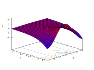
Considering the complex exponential function as a function involving four real variables: the graph of the exponential function is a two-dimensional surface curving through four dimensions.
Starting with a color-coded portion of the domain, the following are depictions of the graph as variously projected into two or three dimensions.
- Graphs of the complex exponential function
-
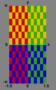 Checker board key:
-
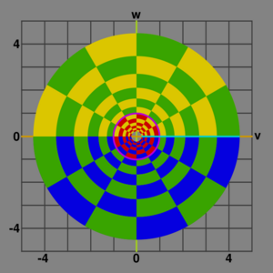 Projection onto the range complex plane (V/W). Compare to the next, perspective picture.
 -
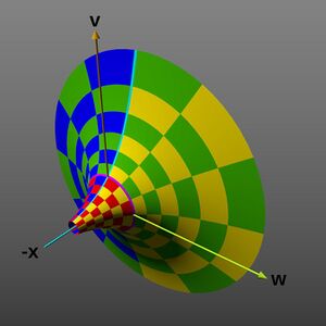 Projection into the , , and dimensions, producing a flared horn or funnel shape (envisioned as 2-D perspective image)
 -
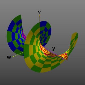 Projection into the , , and dimensions, producing a spiral shape ( range extended to ±2π, again as 2-D perspective image)


The second image shows how the domain complex plane is mapped into the range complex plane:
- zero is mapped to 1
- the real axis is mapped to the positive real axis
- the imaginary axis is wrapped around the unit circle at a constant angular rate
- values with negative real parts are mapped inside the unit circle
- values with positive real parts are mapped outside of the unit circle
- values with a constant real part are mapped to circles centered at zero
- values with a constant imaginary part are mapped to rays extending from zero
The third and fourth images show how the graph in the second image extends into one of the other two dimensions not shown in the second image.
The third image shows the graph extended along the real axis. It shows the graph is a surface of revolution about the axis of the graph of the real exponential function, producing a horn or funnel shape.
The fourth image shows the graph extended along the imaginary axis. It shows that the graph's surface for positive and negative values doesn't really meet along the negative real axis, but instead forms a spiral surface about the axis. Because its values have been extended to ±2π, this image also better depicts the 2π periodicity in the imaginary value.
Matrices and Banach algebras
The power series definition of the exponential function makes sense for square matrices (for which the function is called the matrix exponential) and more generally in any unital Banach algebra B. In this setting, e0 = 1, and ex is invertible with inverse e−x for any x in B. If xy = yx, then ex + y = exey, but this identity can fail for noncommuting x and y.
Some alternative definitions lead to the same function. For instance, ex can be defined as
Or ex can be defined as fx(1), where fx : R → B is the solution to the differential equation dfx/dt(t) = x fx(t), with initial condition fx(0) = 1; it follows that fx(t) = etx for every t in R.
Lie algebras
Given a Lie group G and its associated Lie algebra , the exponential map is a map ↦ G satisfying similar properties. In fact, since R is the Lie algebra of the Lie group of all positive real numbers under multiplication, the ordinary exponential function for real arguments is a special case of the Lie algebra situation. Similarly, since the Lie group GL(n,R) of invertible n × n matrices has as Lie algebra M(n,R), the space of all n × n matrices, the exponential function for square matrices is a special case of the Lie algebra exponential map.
The identity can fail for Lie algebra elements x and y that do not commute; the Baker–Campbell–Hausdorff formula supplies the necessary correction terms.
Transcendency
The function ez is a transcendental function, which means that it is not a root of a polynomial over the ring of the rational fractions
If a1, ..., an are distinct complex numbers, then ea1z, ..., eanz are linearly independent over , and hence ez is transcendental over .
Computation
The Taylor series definition above is generally efficient for computing (an approximation of) . However, when computing near the argument , the result will be close to 1, and computing the value of the difference with floating-point arithmetic may lead to the loss of (possibly all) significant figures, producing a large relative error, possibly even a meaningless result.
Following a proposal by William Kahan, it may thus be useful to have a dedicated routine, often called expm1, which computes ex − 1 directly, bypassing computation of ex. For example,
one may use the Taylor series:
This was first implemented in 1979 in the Hewlett-Packard HP-41C calculator, and provided by several calculators,[17][18] operating systems (for example Berkeley UNIX 4.3BSD[19]), computer algebra systems, and programming languages (for example C99).[20]
In addition to base e, the IEEE 754-2008 standard defines similar exponential functions near 0 for base 2 and 10: and .
A similar approach has been used for the logarithm; see log1p.
An identity in terms of the hyperbolic tangent, gives a high-precision value for small values of x on systems that do not implement expm1(x).
Continued fractions
The exponential function can also be computed with continued fractions.
A continued fraction for ex can be obtained via an identity of Euler:
The following generalized continued fraction for ez, also due to Euler ,[21] converges more quickly:[22]
or, by applying the substitution z = x/y: with a special case for z = 2:
This formula also converges, though more slowly, for z > 2. For example:
See also
- Carlitz exponential, a characteristic p analogue
- Double exponential function – Exponential function of an exponential function
- Exponential field – Mathematical field with an extra operation
- Gaussian function
- Half-exponential function, a compositional square root of an exponential function
- List of exponential topics
- List of integrals of exponential functions
- Mittag-Leffler function, a generalization of the exponential function
- p-adic exponential function
- Padé table for exponential function – Padé approximation of exponential function by a fraction of polynomial functions
- Phase factor
Notes
References
- ↑ "Reviews of Modern Physics Style Guide". XVI.B.1(d): American Physical Society. p. 18. https://cdn.journals.aps.org/files/rmpguide.pdf. "Which form to use, or , is determined by the number of characters and the complexity of the argument. The form is appropriate when the argument is short and simple, i.e., , whereas should be used if the argument is more complicated."
- ↑ T. W. Chaundy; P. R. Barrett; Charles Batey (1954). The Printing of Mathematics. Oxford University Press. p. 31. https://archive.org/details/printingofmathem0000chau/page/31/.
- ↑ "Exponential Function Reference". https://www.mathsisfun.com/sets/function-exponential.html.
- ↑ Real and complex analysis (3rd ed.). New York: McGraw-Hill. 1987. p. 1. ISBN 978-0-07-054234-1. https://archive.org/details/RudinW.RealAndComplexAnalysis3e1987.
- ↑ 5.0 5.1 Weisstein, Eric W.. "Exponential Function" (in en). https://mathworld.wolfram.com/ExponentialFunction.html.
- ↑ Jung, Soon-Mo (2011). "Chapter 9: Exponential Functional Equations". Hyers-Ulam-Rassias Stability of Functional Equations in Nonlinear Analysis. Springer Optimization and Its Applications. 48. Springer New York. pp. 207–225. doi:10.1007/978-1-4419-9637-4_9. ISBN 9781441996374.
- ↑ Aczél, J.; Dhombres, J. (1989). Functional Equations in Several Variables. Encyclopedia of Mathematics and its Applications. 31. Cambridge University Press, Cambridge. p. 10. doi:10.1017/CBO9781139086578. ISBN 0-521-35276-2.
- ↑ 8.0 8.1 e: the Story of a Number. p. 156.
- ↑ G. Harnett, Calculus 1, 1998, Functions continued: "General exponential functions have the property that the ratio of two outputs depends only on the difference of inputs. The ratio of outputs for a unit change in input is the base."
- ↑ G. Harnett, Calculus 1, 1998; Functions continued / Exponentials & logarithms: "The ratio of outputs for a unit change in input is the base of a general exponential function."
- ↑ Serway, Raymond A.; Moses, Clement J.; Moyer, Curt A. (1989). Modern Physics. Fort Worth: Harcourt Brace Jovanovich. p. 384. ISBN 0-03-004844-3.
- ↑ Simmons, George F. (1972). Differential Equations with Applications and Historical Notes. New York: McGraw-Hill. p. 15.
- ↑ "McGraw-Hill Encyclopedia of Science & Technology". McGraw-Hill Encyclopedia of Science & Technology (10th ed.). New York: McGraw-Hill. 2007. ISBN 978-0-07-144143-8.
- ↑ O'Connor, John J.; Robertson, Edmund F., "Exponential function", MacTutor History of Mathematics archive, University of St Andrews, http://www-history.mcs.st-andrews.ac.uk/HistTopics/e.html.
- ↑ Hille, Einar (1959). "The exponential function". Analytic Function Theory. 1. Waltham, MA: Blaisdell. § 6.1, Template:Pgs.
- ↑ Mathematical Analysis (2nd ed.). Reading, Mass.: Addison Wesley. 1974. pp. 19. ISBN 978-0-201-00288-1. https://archive.org/details/mathematicalanal00apos_530.
- ↑ HP 48G Series – Advanced User's Reference Manual (AUR) (4 ed.). Hewlett-Packard. December 1994. HP 00048-90136, 0-88698-01574-2. http://www.hpcalc.org/details.php?id=6036. Retrieved 2015-09-06.
- ↑ HP 50g / 49g+ / 48gII graphing calculator advanced user's reference manual (AUR) (2 ed.). Hewlett-Packard. 2009-07-14. HP F2228-90010. http://www.hpcalc.org/details.php?id=7141. Retrieved 2015-10-10. [1]
- ↑ "Chapter 10.2. Exponential near zero". The Mathematical-Function Computation Handbook - Programming Using the MathCW Portable Software Library (1 ed.). Salt Lake City, UT, USA: Springer International Publishing AG. 2017-08-22. pp. 273–282. doi:10.1007/978-3-319-64110-2. ISBN 978-3-319-64109-6. "Berkeley UNIX 4.3BSD introduced the expm1() function in 1987."
- ↑ "Computation of expm1 = exp(x)−1". Salt Lake City, Utah, USA: Department of Mathematics, Center for Scientific Computing, University of Utah. 2002-07-09. http://www.math.utah.edu/~beebe/reports/expm1.pdf.
- ↑ A. N. Khovanski, The applications of continued fractions and their generalization to problems in approximation theory,1963, Noordhoff, Groningen, The Netherlands
- ↑ "A.2.2 The exponential function.". Continued Fractions. Atlantis Studies in Mathematics. 1. 2008. p. 268. doi:10.2991/978-94-91216-37-4. ISBN 978-94-91216-37-4. https://link.springer.com/content/pdf/bbm%3A978-94-91216-37-4%2F1.
External links
- Hazewinkel, Michiel, ed. (2001), "Exponential function", Encyclopedia of Mathematics, Springer Science+Business Media B.V. / Kluwer Academic Publishers, ISBN 978-1-55608-010-4, https://www.encyclopediaofmath.org/index.php?title=p/e036910
 |  |

