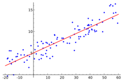
Mean and predicted response
| Part of a series on |
| Regression analysis |
|---|
 |
| Models |
| Estimation |
| Background |
|
|
In linear regression, mean response and predicted response are values of the dependent variable calculated from the regression parameters and a given value of the independent variable. The values of these two responses are the same, but their calculated variances are different.
Background
In straight line fitting, the model is
- [math]\displaystyle{ y_i=\alpha+\beta x_i +\varepsilon_i\, }[/math]
where [math]\displaystyle{ y_i }[/math] is the response variable, [math]\displaystyle{ x_i }[/math] is the explanatory variable, εi is the random error, and [math]\displaystyle{ \alpha }[/math] and [math]\displaystyle{ \beta }[/math] are parameters. The mean, and predicted, response value for a given explanatory value, xd, is given by
- [math]\displaystyle{ \hat{y}_d=\hat\alpha+\hat\beta x_d , }[/math]
while the actual response would be
- [math]\displaystyle{ y_d=\alpha+\beta x_d +\varepsilon_d \, }[/math]
Expressions for the values and variances of [math]\displaystyle{ \hat\alpha }[/math] and [math]\displaystyle{ \hat\beta }[/math] are given in linear regression.
Mean response
Since the data in this context is defined to be (x, y) pairs for every observation, the mean response at a given value of x, say xd, is an estimate of the mean of the y values in the population at the x value of xd, that is [math]\displaystyle{ \hat{E}(y \mid x_d) \equiv\hat{y}_d\! }[/math]. The variance of the mean response is given by
- [math]\displaystyle{ \operatorname{Var}\left(\hat{\alpha} + \hat{\beta}x_d\right) = \operatorname{Var}\left(\hat{\alpha}\right) + \left(\operatorname{Var} \hat{\beta}\right)x_d^2 + 2 x_d \operatorname{Cov} \left(\hat{\alpha}, \hat{\beta} \right) . }[/math]
This expression can be simplified to
- [math]\displaystyle{ \operatorname{Var}\left(\hat{\alpha} + \hat{\beta}x_d\right) =\sigma^2\left(\frac{1}{m} + \frac{\left(x_d - \bar{x}\right)^2}{\sum (x_i - \bar{x})^2}\right), }[/math]
where m is the number of data points.
To demonstrate this simplification, one can make use of the identity
- [math]\displaystyle{ \sum (x_i - \bar{x})^2 = \sum x_i^2 - \frac 1 m \left(\sum x_i\right)^2 . }[/math]
Predicted response
The predicted response distribution is the predicted distribution of the residuals at the given point xd. So the variance is given by
- [math]\displaystyle{ \begin{align} \operatorname{Var}\left(y_d - \left[\hat{\alpha} + \hat{\beta} x_d \right] \right) &= \operatorname{Var} (y_d) + \operatorname{Var} \left(\hat{\alpha} + \hat{\beta}x_d\right) - 2\operatorname{Cov}\left(y_d,\left[\hat{\alpha} + \hat{\beta} x_d \right]\right)\\ &= \operatorname{Var} (y_d) + \operatorname{Var} \left(\hat{\alpha} + \hat{\beta}x_d\right). \end{align} }[/math]
The second line follows from the fact that [math]\displaystyle{ \operatorname{Cov}\left(y_d,\left[\hat{\alpha} + \hat{\beta} x_d \right]\right) }[/math] is zero because the new prediction point is independent of the data used to fit the model. Additionally, the term [math]\displaystyle{ \operatorname{Var} \left(\hat{\alpha} + \hat{\beta}x_d\right) }[/math] was calculated earlier for the mean response.
Since [math]\displaystyle{ \operatorname{Var}(y_d)=\sigma^2 }[/math] (a fixed but unknown parameter that can be estimated), the variance of the predicted response is given by
- [math]\displaystyle{ \begin{align} \operatorname{Var}\left(y_d - \left[\hat{\alpha} + \hat{\beta} x_d \right] \right) & = \sigma^2 + \sigma^2\left(\frac 1 m + \frac{\left(x_d - \bar{x}\right)^2}{\sum (x_i - \bar{x})^2}\right)\\[4pt] & = \sigma^2\left(1 + \frac 1 m + \frac{(x_d - \bar{x})^2}{\sum (x_i - \bar{x})^2}\right). \end{align} }[/math]
Confidence intervals
The [math]\displaystyle{ 100(1-\alpha)\% }[/math] confidence intervals are computed as [math]\displaystyle{ y_d \pm t_{\frac{\alpha }{2},m - n - 1} \sqrt{\operatorname{Var}} }[/math]. Thus, the confidence interval for predicted response is wider than the interval for mean response. This is expected intuitively – the variance of the population of [math]\displaystyle{ y }[/math] values does not shrink when one samples from it, because the random variable εi does not decrease, but the variance of the mean of the [math]\displaystyle{ y }[/math] does shrink with increased sampling, because the variance in [math]\displaystyle{ \hat \alpha }[/math] and [math]\displaystyle{ \hat \beta }[/math] decrease, so the mean response (predicted response value) becomes closer to [math]\displaystyle{ \alpha + \beta x_d }[/math].
This is analogous to the difference between the variance of a population and the variance of the sample mean of a population: the variance of a population is a parameter and does not change, but the variance of the sample mean decreases with increased samples.
General linear regression
The general linear model can be written as
- [math]\displaystyle{ y_i=\sum_{j=1}^n X_{ij}\beta_j + \varepsilon_i\, }[/math]
Therefore, since [math]\displaystyle{ y_d=\sum_{j=1}^n X_{dj}\hat\beta_j }[/math] the general expression for the variance of the mean response is
- [math]\displaystyle{ \operatorname{Var}\left(\sum_{j=1}^n X_{dj}\hat\beta_j\right)= \sum_{i=1}^n \sum_{j=1}^n X_{di}S_{ij}X_{dj}, }[/math]
where S is the covariance matrix of the parameters, given by
- [math]\displaystyle{ \mathbf{S}=\sigma^2\left(\mathbf{X^{\mathsf{T}}X}\right)^{-1}. }[/math]
References
- Draper, N. R.; Smith, H. (1998). Applied Regression Analysis (3rd ed.). John Wiley. ISBN 0-471-17082-8.

