Injective function

Short description: Function that preserves distinctness

"Injective" redirects here. For other uses, see Injective module and Injective object.

In mathematics, an injective function (also known as injection, or one-to-one function) is a function f that maps distinct elements of its domain to distinct elements of its codomain; that is, x₁ ≠ x₂ implies f(x₁) Template:≠ f(x₂) (equivalently by contraposition, f(x₁) = f(x₂) implies x₁ = x₂). In other words, every element of the function's codomain is the image of at most one element of its domain. The term one-to-one function must not be confused with one-to-one correspondence that refers to bijective functions, which are functions such that each element in the codomain is an image of exactly one element in the domain.

A homomorphism between algebraic structures is a function that is compatible with the operations of the structures. For all common algebraic structures, and, in particular for vector spaces, an injective homomorphism is also called a monomorphism. However, in the more general context of category theory, the definition of a monomorphism differs from that of an injective homomorphism. This is thus a theorem that they are equivalent for algebraic structures; see Homomorphism § Monomorphism for more details.

A function $f$ that is not injective is sometimes called many-to-one.

Definition

Template:Dark mode invert Let $f$ be a function whose domain is a set $X$. The function $f$ is said to be injective provided that for all $a$ and $b$ in $X,$ if $f(a)=f(b)$, then $a=b$; that is, $f(a)=f(b)$ implies $a=b$. Equivalently, if $a\ne b$, then $f(a)\ne f(b)$ in the contrapositive statement.

Symbolically,$$\mathrm{\forall }a,b\in X,f(a)=f(b)\Rightarrow a=b,$$ which is logically equivalent to the contrapositive,$$\mathrm{\forall }a,b\in X,a\ne b\Rightarrow f(a)\ne f(b).$$An injective function (or, more generally, a monomorphism) is often denoted by using the specialized arrows ↣ or ↪ (for example, $f:A\rightarrowtail B$ or $f:A\hookrightarrow B$), although some authors specifically reserve ↪ for an inclusion map.

Examples

For visual examples, readers are directed to the gallery section.

• For any set $X$ and any subset $S\subseteq X$, the inclusion map $S\to X$ (which sends any element $s\in S$ to itself) is injective. In particular, the identity function $X\to X$ is always injective (and in fact bijective).
• If the domain of a function is the empty set, then the function is the empty function, which is injective.
• If the domain of a function has one element (that is, it is a singleton set), then the function is always injective.
• The function $f:\mathbb{ℝ}\to \mathbb{ℝ}$ defined by $f(x)=2x+1$ is injective.
• The function $g:\mathbb{ℝ}\to \mathbb{ℝ}$ defined by $g(x)=x^2$ is not injective, because (for example) $g(1)=1=g(-1).$ However, if $g$ is redefined so that its domain is the non-negative real numbers [0, +∞), then $g$ is injective.
• The exponential function $\exp :\mathbb{ℝ}\to \mathbb{ℝ}$ defined by $\exp (x)=e^x$ is injective (but not surjective, as no real value maps to a negative number).
• The natural logarithm function $\ln :(0,\mathrm{\infty })\to \mathbb{ℝ}$ defined by $x\mapsto \ln x$ is injective.
• The function $g:\mathbb{ℝ}\to \mathbb{ℝ}$ defined by $g(x)=x^n-x$ is not injective, since, for example, $g(0)=g(1)=0$.

More generally, when $X$ and $Y$ are both the real line $\mathbb{ℝ}$, then an injective function $f:\mathbb{ℝ}\to \mathbb{ℝ}$ is one whose graph is never intersected by any horizontal line more than once. This principle is referred to as the horizontal line test.

Injections can be undone

Functions with left inverses are always injections. That is, given $f:X\to Y$, if there is a function $g:Y\to X$ such that for every $x\in X$, $g(f(x))=x$, then $f$ is injective. The proof is that $$f(a)=f(b)\to g(f(a))=g(f(b))\to a=b.$$

In this case, $g$ is called a retraction of $f$. Conversely, $f$ is called a section of $g$. For example: $f:\mathbb{ℝ}\to {\mathbb{ℝ}}^2,x\mapsto (1,m{)}^{⊺}x$ is retracted by $g:y\mapsto \frac{(1,m)}{1+m^2}y$.

Conversely, every injection $f$ with a non-empty domain has a left inverse $g$. It can be defined by choosing an element $a$ in the domain of $f$ and setting $g(y)$ to the unique element of the pre-image $f^{-1}[y]$ (if it is non-empty) or to $a$ (otherwise).

The left inverse $g$ is not necessarily an inverse of $f,$ because the composition in the other order, $f\circ g$, may differ from the identity on $Y$. In other words, an injective function can be "reversed" by a left inverse, but is not necessarily invertible, which requires that the function is bijective.

Injections may be made invertible

In fact, to turn an injective function $f:X\to Y$ into a bijective (hence invertible) function, it suffices to replace its codomain $Y$ by its actual image $J=f(X).$ That is, let $g:X\to J$ such that $g(x)=f(x)$ for all $x\in X$; then $g$ is bijective. Indeed, $f$ can be factored as ${\mathrm{In}}_{J,Y}\circ g$, where ${\mathrm{In}}_{J,Y}$ is the inclusion function from $J$ into $Y$.

More generally, injective partial functions are called partial bijections.

Other properties

• If $f$ and $g$ are both injective then $f\circ g$ is injective.
• If $g\circ f$ is injective, then $f$ is injective (but $g$ need not be).
• $f:X\to Y$ is injective if and only if, given any functions $g$, $h:W\to X$ whenever $f\circ g=f\circ h$, then $g=h$. In other words, injective functions are precisely the monomorphisms in the category Set of sets.
• If $f:X\to Y$ is injective and $A$ is a subset of $X$, then $f^{-1}(f(A))=A$. Thus, $A$ can be recovered from its image $f(A)$.
• If $f:X\to Y$ is injective and $A$ and $B$ are both subsets of $X$, then $f(A\cap B)=f(A)\cap f(B)$.
• Every function $h:W\to Y$ can be decomposed as $h=f\circ g$ for a suitable injection $f$ and surjection $g$. This decomposition is unique up to isomorphism, and $f$ may be thought of as the inclusion function of the range $h(W)$ of $h$ as a subset of the codomain $Y$ of $h$.
• If $f:X\to Y$ is an injective function, then $Y$ has at least as many elements as $X,$ in the sense of cardinal numbers. In particular, if, in addition, there is an injection from $Y$ to $X$, then $X$ and $Y$ have the same cardinal number. (This is known as the Cantor–Bernstein–Schroeder theorem.)
• If both $X$ and $Y$ are finite with the same number of elements, then $f:X\to Y$ is injective if and only if $f$ is surjective (in which case $f$ is bijective).
• An injective function which is a homomorphism between two algebraic structures is an embedding.
• Unlike surjectivity, which is a relation between the graph of a function and its codomain, injectivity is a property of the graph of the function alone; that is, whether a function $f$ is injective can be decided by only considering the graph (and not the codomain) of $f$.

Proving that functions are injective

A proof that a function $f$ is injective depends on how the function is presented and what properties the function holds. For functions that are given by some formula there is a basic idea. We use the definition of injectivity, namely that if $f(x)=f(y)$, then $x=y$.

Here is an example: $$f(x)=2x+3$$

Proof: Let $f:X\to Y$. Suppose $f(x)=f(y)$. So $2x+3=2y+3$ implies $2x=2y$, which implies $x=y$. Therefore, it follows from the definition that $f$ is injective.

There are multiple other methods of proving that a function is injective. For example, in calculus if $f$ is a differentiable function defined on some interval, then it is sufficient to show that the derivative is always positive or always negative on that interval. In linear algebra, if $f$ is a linear transformation it is sufficient to show that the kernel of $f$ contains only the zero vector. If $f$ is a function with finite domain it is sufficient to look through the list of images of each domain element and check that no image occurs twice on the list.

A graphical approach for a real-valued function $f$ of a real variable $x$ is the horizontal line test. If every horizontal line intersects the curve of $f(x)$ in at most one point, then $f$ is injective or one-to-one.

Gallery

• 
  An injective non-surjective function (injection, not a bijection)
• 
  An injective surjective function (bijection)
• 
  A non-injective surjective function (surjection, not a bijection)
• 
  A non-injective non-surjective function (also not a bijection)

• 
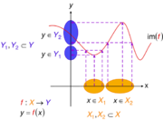  Not an injective function. Here $X_1$ and $X_2$ are subsets of $X,Y_1$ and $Y_2$ are subsets of $Y$: for two regions where the function is not injective because more than one domain element can map to a single range element. That is, it is possible for more than one $x$ in $X$ to map to the same $y$ in $Y$.
• 
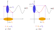  Making functions injective. The previous function $f:X\to Y$ can be reduced to one or more injective functions (say) $f:X_1\to Y_1$ and $f:X_2\to Y_2$, shown by solid curves (long-dash parts of initial curve are not mapped to anymore). Notice how the rule $f$ has not changed – only the domain and range. $X_1$ and $X_2$ are subsets of $X,Y_1$ and $Y_2$ are subsets of $Y$: for two regions where the initial function can be made injective so that one domain element can map to a single range element. That is, only one $x$ in $X$ maps to one $y$ in $Y$.
• 
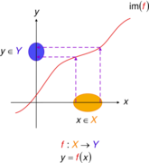  Injective functions. Diagramatic interpretation in the Cartesian plane, defined by the mapping $f:X\to Y$, where $y=f(x)$, $X=$ domain of function, $Y=$ range of function, and $\mathrm{im}(f)$ denotes image of $f$. Every one $x$ in $X$ maps to exactly one unique $y$ in $Y$. The circled parts of the axes represent domain and range sets — in accordance with the standard diagrams above

See also

• Bijection, injection and surjection – Properties of mathematical functions
• Injective metric space – Type of metric space
• Monotonic function – Order-preserving mathematical function
• Univalent function – Mathematical concept

References

• Bartle, Robert G. (1976), The Elements of Real Analysis (2nd ed.), New York: John Wiley & Sons, ISBN 978-0-471-05464-1 , p. 17 ff.
• Halmos, Paul R. (1974), Naive Set Theory, New York: Springer, ISBN 978-0-387-90092-6 , p. 38 ff.

External links

• Earliest Uses of Some of the Words of Mathematics: entry on Injection, Surjection and Bijection has the history of Injection and related terms.
• Khan Academy – Surjective (onto) and Injective (one-to-one) functions: Introduction to surjective and injective functions