Variance of the mean and predicted responses
| Part of a series on |
| Regression analysis |
|---|
 |
| Models |
| Estimation |
| Background |
|
|
In regression, mean response (or expected response) and predicted response, also known as mean outcome (or expected outcome) and predicted outcome, are values of the dependent variable calculated from the regression parameters and a given value of the independent variable. The values of these two responses are the same, but their calculated variances are different. The concept is a generalization of the distinction between the standard error of the mean and the sample standard deviation.
Background: simple linear regression
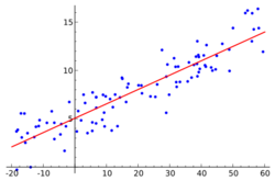
In simple linear regression (i.e., straight line fitting with errors only in the y-coordinate), the model is
where is the response variable, is the explanatory variable, εi is the random error, and and are parameters. The mean, and predicted, response value for a given explanatory value, xd, is given by
while the actual response would be
Expressions for the values and variances of and are given in linear regression.
Variance
Variance of the mean response
Since the data in this context is defined to be (x, y) pairs for every observation, the mean response at a given value of x, say xd, is an estimate of the mean of the y values in the population at the x value of xd, that is . The variance of the mean response is given by
This expression can be simplified to
where m is the number of data points.
To demonstrate this simplification, one can make use of the identity
Variance of the predicted response
The predicted response distribution is the predicted distribution of the residuals at the given point xd. So the variance is given by
The second line follows from the fact that is zero because the new prediction point is independent of the data used to fit the model. Additionally, the term was calculated earlier for the mean response.
Since (a fixed but unknown parameter that can be estimated), the variance of the predicted response is given by
Confidence intervals
The confidence intervals are computed as . Thus, the confidence interval for predicted response is wider than the interval for mean response. This is expected intuitively – the variance of the population of values does not shrink when one samples from it, because the random variable εi does not decrease, but the variance of the mean of the does shrink with increased sampling, because the variance in and decrease, so the mean response (predicted response value) becomes closer to .
This is analogous to the difference between the variance of a population and the variance of the sample mean of a population: the variance of a population is a parameter and does not change, but the variance of the sample mean decreases with increased sample size.
General case
The general case of linear regression can be written as
Therefore, since the general expression for the variance of the mean response is
where S is the covariance matrix of the parameters, given by
See also
- Expected value
- Prediction error
- Regression prediction
References
- Draper, N. R.; Smith, H. (1998). Applied Regression Analysis (3rd ed.). John Wiley. ISBN 0-471-17082-8.
 |
