Conway polyhedron notation

In geometry, Conway polyhedron notation, invented by John Horton Conway and promoted by George W. Hart, is used to describe polyhedra based on a seed polyhedron modified by various prefix operations.[1][2]
Conway and Hart extended the idea of using operators, like truncation as defined by Kepler, to build related polyhedra of the same symmetry. For example, tC represents a truncated cube, and taC, parsed as t(aC), is (topologically) a truncated cuboctahedron. The simplest operator dual swaps vertex and face elements; e.g., a dual cube is an octahedron: dC = O. Applied in a series, these operators allow many higher order polyhedra to be generated. Conway defined the operators a (ambo), b (bevel), d (dual), e (expand), g (gyro), j (join), k (kis), m (meta), o (ortho), s (snub), and t (truncate), while Hart added r (reflect) and p (propellor).[3] Later implementations named further operators, sometimes referred to as "extended" operators.[4][5] Conway's basic operations are sufficient to generate the Archimedean and Catalan solids from the Platonic solids. Some basic operations can be made as composites of others: for instance, ambo applied twice is the expand operation (aa = e), while a truncation after ambo produces bevel (ta = b).
Polyhedra can be studied topologically, in terms of how their vertices, edges, and faces connect together, or geometrically, in terms of the placement of those elements in space. Different implementations of these operators may create polyhedra that are geometrically different but topologically equivalent. These topologically equivalent polyhedra can be thought of as one of many embeddings of a polyhedral graph on the sphere. Unless otherwise specified, in this article (and in the literature on Conway operators in general) topology is the primary concern. Polyhedra with genus 0 (i.e. topologically equivalent to a sphere) are often put into canonical form to avoid ambiguity.
Operators
In Conway's notation, operations on polyhedra are applied like functions, from right to left. For example, a cuboctahedron is an ambo cube,[6] i.e. [math]\displaystyle{ a(C) = aC }[/math], and a truncated cuboctahedron is [math]\displaystyle{ t(a(C)) = t(aC) = taC }[/math]. Repeated application of an operator can be denoted with an exponent: j2 = o. In general, Conway operators are not commutative.
Individual operators can be visualized in terms of fundamental domains (or chambers), as below. Each right triangle is a fundamental domain. Each white chamber is a rotated version of the others, and so is each colored chamber. For achiral operators, the colored chambers are a reflection of the white chambers, and all are transitive. In group terms, achiral operators correspond to dihedral groups Dn where n is the number of sides of a face, while chiral operators correspond to cyclic groups Cn lacking the reflective symmetry of the dihedral groups. Achiral and chiral operators are also called local symmetry-preserving operations (LSP) and local operations that preserve orientation-preserving symmetries (LOPSP), respectively.[7][8][9] LSPs should be understood as local operations that preserve symmetry, not operations that preserve local symmetry. Again, these are symmetries in a topological sense, not a geometric sense: the exact angles and edge lengths may differ.
| 3 (Triangle) | 4 (Square) | 5 (Pentagon) | 6 (Hexagon) |
|---|---|---|---|

|

|

|

|
| The fundamental domains for polyhedron groups. The groups are [math]\displaystyle{ D_3,D_4,D_5,D_6 }[/math] for achiral polyhedra, and [math]\displaystyle{ C_3,C_4,C_5,C_6 }[/math] for chiral polyhedra. | |||
Hart introduced the reflection operator r, that gives the mirror image of the polyhedron.[6] This is not strictly a LOPSP, since it does not preserve orientation: it reverses it, by exchanging white and red chambers. r has no effect on achiral polyhedra aside from orientation, and rr = S returns the original polyhedron. An overline can be used to indicate the other chiral form of an operator: s = rsr.
An operation is irreducible if it cannot be expressed as a composition of operators aside from d and r. The majority of Conway's original operators are irreducible: the exceptions are e, b, o, and m.
Matrix representation
| x | [math]\displaystyle{ \begin{bmatrix} a & b & c \\ 0 & d & 0 \\ a' & b' & c' \end{bmatrix}=\mathbf{M}_x }[/math] |
|---|---|
| xd | [math]\displaystyle{ \begin{bmatrix} c & b & a \\ 0 & d & 0 \\ c' & b' & a' \end{bmatrix}=\mathbf{M}_x\mathbf{M}_d }[/math] |
| dx | [math]\displaystyle{ \begin{bmatrix} a' & b' & c' \\ 0 & d & 0 \\ a & b & c \end{bmatrix}=\mathbf{M}_d\mathbf{M}_x }[/math] |
| dxd | [math]\displaystyle{ \begin{bmatrix} c' & b' & a' \\ 0 & d & 0 \\ c & b & a \end{bmatrix} = \mathbf{M}_d\mathbf{M}_x\mathbf{M}_d }[/math] |
The relationship between the number of vertices, edges, and faces of the seed and the polyhedron created by the operations listed in this article can be expressed as a matrix [math]\displaystyle{ \mathbf{M}_x }[/math]. When x is the operator, [math]\displaystyle{ v,e,f }[/math] are the vertices, edges, and faces of the seed (respectively), and [math]\displaystyle{ v',e',f' }[/math] are the vertices, edges, and faces of the result, then
- [math]\displaystyle{ \mathbf{M}_x \begin{bmatrix} v \\ e \\ f \end{bmatrix} = \begin{bmatrix} v' \\ e' \\ f' \end{bmatrix} }[/math].
The matrix for the composition of two operators is just the product of the matrixes for the two operators. Distinct operators may have the same matrix, for example, p and l. The edge count of the result is an integer multiple d of that of the seed: this is called the inflation rate, or the edge factor.[7]
The simplest operators, the identity operator S and the dual operator d, have simple matrix forms:
- [math]\displaystyle{ \mathbf{M}_S = \begin{bmatrix} 1 & 0 & 0 \\ 0 & 1 & 0 \\ 0 & 0 & 1 \end{bmatrix} = \mathbf{I}_3 }[/math], [math]\displaystyle{ \mathbf{M}_d = \begin{bmatrix} 0 & 0 & 1 \\ 0 & 1 & 0 \\ 1 & 0 & 0 \end{bmatrix} }[/math]
Two dual operators cancel out; dd = S, and the square of [math]\displaystyle{ \mathbf{M}_d }[/math] is the identity matrix. When applied to other operators, the dual operator corresponds to horizontal and vertical reflections of the matrix. Operators can be grouped into groups of four (or fewer if some forms are the same) by identifying the operators x, xd (operator of dual), dx (dual of operator), and dxd (conjugate of operator). In this article, only the matrix for x is given, since the others are simple reflections.
Number of operators
The number of LSPs for each inflation rate is [math]\displaystyle{ 2, 2, 4, 6, 6, 20, 28, 58, 82, \cdots }[/math] starting with inflation rate 1. However, not all LSPs necessarily produce a polyhedron whose edges and vertices form a 3-connected graph, and as a consequence of Steinitz's theorem do not necessarily produce a convex polyhedron from a convex seed. The number of 3-connected LSPs for each inflation rate is [math]\displaystyle{ 2, 2, 4, 6, 4, 20, 20, 54, 64, \cdots }[/math].[8]
Original operations
Strictly, seed (S), needle (n), and zip (z) were not included by Conway, but they are related to original Conway operations by duality so are included here.
From here on, operations are visualized on cube seeds, drawn on the surface of that cube. Blue faces cross edges of the seed, and pink faces lie over vertices of the seed. There is some flexibility in the exact placement of vertices, especially with chiral operators.
| Edge factor | Matrix [math]\displaystyle{ \mathbf{M}_x }[/math] | x | xd | dx | dxd | Notes |
|---|---|---|---|---|---|---|
| 1 | [math]\displaystyle{ \begin{bmatrix} 1 & 0 & 0 \\ 0 & 1 & 0 \\ 0 & 0 & 1 \end{bmatrix} }[/math] |  Seed: S |
 Dual: d |
Seed: dd = S |
Dual replaces each face with a vertex, and each vertex with a face. | |
| 2 | [math]\displaystyle{ \begin{bmatrix} 1 & 0 & 1 \\ 0 & 2 & 0 \\ 0 & 1 & 0 \end{bmatrix} }[/math] |  Join: j |
 Ambo: a |
Join creates quadrilateral faces. Ambo creates degree-4 vertices, and is also called rectification, or the medial graph in graph theory.[10] | ||
| 3 | [math]\displaystyle{ \begin{bmatrix} 1 & 0 & 1 \\ 0 & 3 & 0 \\ 0 & 2 & 0 \end{bmatrix} }[/math] |  Kis: k |
 Needle: n |
 Zip: z |
 Truncate: t |
Kis raises a pyramid on each face, and is also called akisation, Kleetope, cumulation,[11] accretion, or pyramid-augmentation. Truncate cuts off the polyhedron at its vertices but leaves a portion of the original edges.[12] Zip is also called bitruncation. |
| 4 | [math]\displaystyle{ \begin{bmatrix} 1 & 1 & 1 \\ 0 & 4 & 0 \\ 0 & 2 & 0 \end{bmatrix} }[/math] |  Ortho: o = jj |
 Expand: e = aa |
|||
| 5 | [math]\displaystyle{ \begin{bmatrix} 1 & 2 & 1 \\ 0 & 5 & 0 \\ 0 & 2 & 0 \end{bmatrix} }[/math] |  Gyro: g |
gd = rgr | sd = rsr |  Snub: s |
Chiral operators. See Snub (geometry). Contrary to Hart,[3] gd is not the same as g: it is its chiral pair.[13] |
| 6 | [math]\displaystyle{ \begin{bmatrix} 1 & 1 & 1 \\ 0 & 6 & 0 \\ 0 & 4 & 0 \end{bmatrix} }[/math] |  Meta: m = kj |
 Bevel: b = ta |
|||
Seeds
Any polyhedron can serve as a seed, as long as the operations can be executed on it. Common seeds have been assigned a letter. The Platonic solids are represented by the first letter of their name (Tetrahedron, Octahedron, Cube, Icosahedron, Dodecahedron); the prisms (Pn) for n-gonal forms; antiprisms (An); cupolae (Un); anticupolae (Vn); and pyramids (Yn). Any Johnson solid can be referenced as Jn, for n=1..92.
All of the five Platonic solids can be generated from prismatic generators with zero to two operators:[14]
- Triangular pyramid: Y3 (A tetrahedron is a special pyramid)
- Triangular antiprism: A3 (An octahedron is a special antiprism)
- O = A3
- C = dA3
- Square prism: P4 (A cube is a special prism)
- C = P4
- Pentagonal antiprism: A5
- I = k5A5 (A special gyroelongated dipyramid)
- D = t5dA5 (A special truncated trapezohedron)
The regular Euclidean tilings can also be used as seeds:
- Q = Quadrille = Square tiling
- H = Hextille = Hexagonal tiling = dΔ
- Δ = Deltille = Triangular tiling = dH
Extended operations
These are operations created after Conway's original set. Note that many more operations exist than have been named; just because an operation is not here does not mean it does not exist (or is not an LSP or LOPSP). To simplify, only irreducible operators are included in this list: others can be created by composing operators together.
| Edge factor | Matrix [math]\displaystyle{ \mathbf{M}_x }[/math] | x | xd | dx | dxd | Notes |
|---|---|---|---|---|---|---|
| 4 | [math]\displaystyle{ \begin{bmatrix} 1 & 2 & 0 \\ 0 & 4 & 0 \\ 0 & 1 & 1 \end{bmatrix} }[/math] |  Chamfer: c |
 cd = du |
 dc = ud |
 Subdivide: u |
Chamfer is the join-form of l. See Chamfer (geometry). |
| 5 | [math]\displaystyle{ \begin{bmatrix} 1 & 2 & 0 \\ 0 & 5 & 0 \\ 0 & 2 & 1 \end{bmatrix} }[/math] |  Propeller: p |
 dp = pd |
dpd = p |
Chiral operators. The propeller operator was developed by George Hart.[15] | |
| 5 | [math]\displaystyle{ \begin{bmatrix} 1 & 2 & 0 \\ 0 & 5 & 0 \\ 0 & 2 & 1 \end{bmatrix} }[/math] |  Loft: l |
 ld |
 dl |
 dld |
|
| 6 | [math]\displaystyle{ \begin{bmatrix} 1 & 3 & 0 \\ 0 & 6 & 0 \\ 0 & 2 & 1 \end{bmatrix} }[/math] |  Quinto: q |
 qd |
 dq |
 dqd |
|
| 6 | [math]\displaystyle{ \begin{bmatrix} 1 & 2 & 0 \\ 0 & 6 & 0 \\ 0 & 3 & 1 \end{bmatrix} }[/math] |  Join-lace: L0 |
 L0d |
 dL0 |
 dL0d |
See below for explanation of join notation. |
| 7 | [math]\displaystyle{ \begin{bmatrix} 1 & 2 & 0 \\ 0 & 7 & 0 \\ 0 & 4 & 1 \end{bmatrix} }[/math] |  Lace: L |
 Ld |
 dL |
 dLd |
|
| 7 | [math]\displaystyle{ \begin{bmatrix} 1 & 2 & 1 \\ 0 & 7 & 0 \\ 0 & 4 & 0 \end{bmatrix} }[/math] |  Stake: K |
 Kd |
 dK |
 dKd |
|
| 7 | [math]\displaystyle{ \begin{bmatrix} 1 & 4 & 0 \\ 0 & 7 & 0 \\ 0 & 2 & 1 \end{bmatrix} }[/math] |  Whirl: w |
wd = dv |  vd = dw |
Volute: v | Chiral operators. |
| 8 | [math]\displaystyle{ \begin{bmatrix} 1 & 2 & 1 \\ 0 & 8 & 0 \\ 0 & 5 & 0 \end{bmatrix} }[/math] | 0C.png) Join-kis-kis: [math]\displaystyle{ (kk)_0 }[/math] |
0dC.png) [math]\displaystyle{ (kk)_0d }[/math] |
0C.png) [math]\displaystyle{ d(kk)_0 }[/math] |
0dC.png) [math]\displaystyle{ d(kk)_0d }[/math] |
Sometimes named J.[4] See below for explanation of join notation. The non-join-form, kk, is not irreducible. |
| 10 | [math]\displaystyle{ \begin{bmatrix} 1 & 3 & 1 \\ 0 & 10 & 0 \\ 0 & 6 & 0 \end{bmatrix} }[/math] |  Cross: X |
 Xd |
 dX |
 dXd |
|
Indexed extended operations
A number of operators can be grouped together by some criteria, or have their behavior modified by an index.[4] These are written as an operator with a subscript: xn.
Augmentation
Augmentation operations retain original edges. They may be applied to any independent subset of faces, or may be converted into a join-form by removing the original edges. Conway notation supports an optional index to these operators: 0 for the join-form, or 3 or higher for how many sides affected faces have. For example, k4Y4=O: taking a square-based pyramid and gluing another pyramid to the square base gives an octahedron.
| Operator | k | l | L | K | (kk) |
|---|---|---|---|---|---|
| x |
|
|
|
|

|
| x0 | k0 = j |
l0 = c |
L0 |
 K0 = jk |
[math]\displaystyle{ (kk)_0 }[/math] |
| Augmentation | Pyramid | Prism | Antiprism |
The truncate operator t also has an index form tn, indicating that only vertices of a certain degree are truncated. It is equivalent to dknd.
Some of the extended operators can be created in special cases with kn and tn operators. For example, a chamfered cube, cC, can be constructed as t4daC, as a rhombic dodecahedron, daC or jC, with its degree-4 vertices truncated. A lofted cube, lC is the same as t4kC. A quinto-dodecahedron, qD can be constructed as t5daaD or t5deD or t5oD, a deltoidal hexecontahedron, deD or oD, with its degree-5 vertices truncated.
Meta/Bevel
Meta adds vertices at the center and along the edges, while bevel adds faces at the center, seed vertices, and along the edges. The index is how many vertices or faces are added along the edges. Meta (in its non-indexed form) is also called cantitruncation or omnitruncation. Note that 0 here does not mean the same as for augmentation operations: it means zero vertices (or faces) are added along the edges.[4]
| n | Edge factor | Matrix [math]\displaystyle{ \mathbf{M}_x }[/math] | x | xd | dx | dxd |
|---|---|---|---|---|---|---|
| 0 | 3 | [math]\displaystyle{ \begin{bmatrix} 1 & 0 & 1 \\ 0 & 3 & 0 \\ 0 & 2 & 0 \end{bmatrix} }[/math] | k = m0 |
n |
z = b0 |
t |
| 1 | 6 | [math]\displaystyle{ \begin{bmatrix} 1 & 1 & 1 \\ 0 & 6 & 0 \\ 0 & 4 & 0 \end{bmatrix} }[/math] | m = m1 = kj |
b = b1 = ta | ||
| 2 | 9 | [math]\displaystyle{ \begin{bmatrix} 1 & 2 & 1 \\ 0 & 9 & 0 \\ 0 & 6 & 0 \end{bmatrix} }[/math] |  m2 |
 m2d |
 b2 |
 b2d |
| 3 | 12 | [math]\displaystyle{ \begin{bmatrix} 1 & 3 & 1 \\ 0 & 12 & 0 \\ 0 & 8 & 0 \end{bmatrix} }[/math] |  m3 |
m3d | b3 | b3d |
| n | 3n+3 | [math]\displaystyle{ \begin{bmatrix} 1 & n & 1 \\ 0 & 3n+3 & 0 \\ 0 & 2n+2 & 0 \end{bmatrix} }[/math] | mn | mnd | bn | bnd |
Medial
Medial is like meta, except it does not add edges from the center to each seed vertex. The index 1 form is identical to Conway's ortho and expand operators: expand is also called cantellation and expansion. Note that o and e have their own indexed forms, described below. Also note that some implementations start indexing at 0 instead of 1.[4]
| n | Edge factor |
Matrix [math]\displaystyle{ \mathbf{M}_x }[/math] | x | xd | dx | dxd |
|---|---|---|---|---|---|---|
| 1 | 4 | [math]\displaystyle{ \begin{bmatrix} 1 & 1 & 1 \\ 0 & 4 & 0 \\ 0 & 2 & 0 \end{bmatrix} }[/math] | M1 = o = jj |
e = aa | ||
| 2 | 7 | [math]\displaystyle{ \begin{bmatrix} 1 & 2 & 1 \\ 0 & 7 & 0 \\ 0 & 4 & 0 \end{bmatrix} }[/math] |  Medial: M = M2 |
 Md |
 dM |
 dMd |
| n | 3n+1 | [math]\displaystyle{ \begin{bmatrix} 1 & n & 1 \\ 0 & 3n+1 & 0 \\ 0 & 2n & 0 \end{bmatrix} }[/math] | Mn | Mnd | dMn | dMnd |
Goldberg-Coxeter
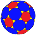
The Goldberg-Coxeter (GC) Conway operators are two infinite families of operators that are an extension of the Goldberg-Coxeter construction.[16][17] The GC construction can be thought of as taking a triangular section of a triangular lattice, or a square section of a square lattice, and laying that over each face of the polyhedron. This construction can be extended to any face by identifying the chambers of the triangle or square (the "master polygon").[7] Operators in the triangular family can be used to produce the Goldberg polyhedra and geodesic polyhedra: see List of geodesic polyhedra and Goldberg polyhedra for formulas.
The two families are the triangular GC family, ca,b and ua,b, and the quadrilateral GC family, ea,b and oa,b. Both the GC families are indexed by two integers [math]\displaystyle{ a \ge 1 }[/math] and [math]\displaystyle{ b \ge 0 }[/math]. They possess many nice qualities:
- The indexes of the families have a relationship with certain Euclidean domains over the complex numbers: the Eisenstein integers for the triangular GC family, and the Gaussian integers for the quadrilateral GC family.
- Operators in the x and dxd columns within the same family commute with each other.
The operators are divided into three classes (examples are written in terms of c but apply to all 4 operators):
- Class I: [math]\displaystyle{ b=0 }[/math]. Achiral, preserves original edges. Can be written with the zero index suppressed, e.g. ca,0 = ca.
- Class II: [math]\displaystyle{ a=b }[/math]. Also achiral. Can be decomposed as ca,a = cac1,1
- Class III: All other operators. These are chiral, and ca,b and cb,a are the chiral pairs of each other.
Of the original Conway operations, the only ones that do not fall into the GC family are g and s (gyro and snub). Meta and bevel (m and b) can be expressed in terms of one operator from the triangular family and one from the quadrilateral family.
Triangular
| a | b | Class | Edge factor T = a2 + ab + b2 |
Matrix [math]\displaystyle{ \mathbf{M}_x }[/math] | Master triangle | x | xd | dx | dxd |
|---|---|---|---|---|---|---|---|---|---|
| 1 | 0 | I | 1 | [math]\displaystyle{ \begin{bmatrix} 1 & 0 & 0 \\ 0 & 1 & 0 \\ 0 & 0 & 1 \end{bmatrix} }[/math] | 
|
u1 = S |
d |
c1 = S | |
| 2 | 0 | I | 4 | [math]\displaystyle{ \begin{bmatrix} 1 & 1 & 0 \\ 0 & 4 & 0 \\ 0 & 2 & 1 \end{bmatrix} }[/math] | 
|
u2 = u |
dc |
du |
c2 = c |
| 3 | 0 | I | 9 | [math]\displaystyle{ \begin{bmatrix} 1 & 2 & 1 \\ 0 & 9 & 0 \\ 0 & 6 & 0 \end{bmatrix} }[/math] | 
|
 u3 = nn |
 nk |
 zt |
 c3 = zz |
| 4 | 0 | I | 16 | [math]\displaystyle{ \begin{bmatrix} 1 & 5 & 0 \\ 0 & 16 & 0 \\ 0 & 10 & 1 \end{bmatrix} }[/math] | 
|
 u4 = uu |
uud = dcc | duu = ccd | c4 = cc |
| 5 | 0 | I | 25 | [math]\displaystyle{ \begin{bmatrix} 1 & 8 & 0 \\ 0 & 25 & 0 \\ 0 & 16 & 1 \end{bmatrix} }[/math] | 
|
 u5 |
u5d = dc5 | du5 = c5d | c5 |
| 6 | 0 | I | 36 | [math]\displaystyle{ \begin{bmatrix} 1 & 11 & 1 \\ 0 & 36 & 0 \\ 0 & 24 & 0 \end{bmatrix} }[/math] | 
|
 u6 = unn |
unk | czt | u6 = czz |
| 7 | 0 | I | 49 | [math]\displaystyle{ \begin{bmatrix} 1 & 16 & 0 \\ 0 & 49 & 0 \\ 0 & 32 & 1 \end{bmatrix} }[/math] | 
|
 u7 = u2,1u1,2 = vrv |
vrvd = dwrw | dvrv = wrwd | c7 = c2,1c1,2 = wrw |
| 8 | 0 | I | 64 | [math]\displaystyle{ \begin{bmatrix} 1 & 21 & 0 \\ 0 & 64 & 0 \\ 0 & 42 & 1 \end{bmatrix} }[/math] | 
|
 u8 = u3 |
u3d = dc3 | du3 = c3d | c8 = c3 |
| 9 | 0 | I | 81 | [math]\displaystyle{ \begin{bmatrix} 1 & 26 & 1 \\ 0 & 81 & 0 \\ 0 & 54 & 0 \end{bmatrix} }[/math] | 
|
 u9 = n4 |
n3k = kz3 | tn3 = z3t | c9 = z4 |
| 1 | 1 | II | 3 | [math]\displaystyle{ \begin{bmatrix} 1 & 0 & 1 \\ 0 & 3 & 0 \\ 0 & 2 & 0 \end{bmatrix} }[/math] | 
|
u1,1 = n |
k |
t |
c1,1 = z |
| 2 | 1 | III | 7 | [math]\displaystyle{ \begin{bmatrix} 1 & 2 & 0 \\ 0 & 7 & 0 \\ 0 & 4 & 1 \end{bmatrix} }[/math] | 
|
v = u2,1 | vd = dw |
dv = wd | w = c2,1 |
| 3 | 1 | III | 13 | [math]\displaystyle{ \begin{bmatrix} 1 & 4 & 0 \\ 0 & 13 & 0 \\ 0 & 8 & 1 \end{bmatrix} }[/math] | 
|
u3,1 | u3,1d = dc3,1 | du3,1 = c3,1d |  c3,1 |
| 3 | 2 | III | 19 | [math]\displaystyle{ \begin{bmatrix} 1 & 6 & 0 \\ 0 & 19 & 0 \\ 0 & 12 & 1 \end{bmatrix} }[/math] | 
|
u3,2 | u3,2d = dc3,2 | du3,2 = c3,2d |  c3,2 |
| 4 | 3 | III | 37 | [math]\displaystyle{ \begin{bmatrix} 1 & 12 & 0 \\ 0 & 37 & 0 \\ 0 & 24 & 1 \end{bmatrix} }[/math] | 
|
u4,3 | u4,3d = dc4,3 | du4,3 = c4,3d |  c4,3 |
| 5 | 4 | III | 61 | [math]\displaystyle{ \begin{bmatrix} 1 & 20 & 0 \\ 0 & 61 & 0 \\ 0 & 40 & 1 \end{bmatrix} }[/math] | 
|
u5,4 | u5,4d = dc5,4 | du5,4 = c5,4d |  c5,4 |
| 6 | 5 | III | 91 | [math]\displaystyle{ \begin{bmatrix} 1 & 30 & 0 \\ 0 & 91 & 0 \\ 0 & 60 & 1 \end{bmatrix} }[/math] | 
|
u6,5 = u1,2u1,3 | u6,5d = dc6,5 | du6,5 = c6,5d |  c6,5=c1,2c1,3 |
| 7 | 6 | III | 127 | [math]\displaystyle{ \begin{bmatrix} 1 & 42 & 0 \\ 0 & 127 & 0 \\ 0 & 84 & 1 \end{bmatrix} }[/math] | 
|
u7,6 | u7,6d = dc7,6 | du7,6 = c7,6d |  c7,6 |
| 8 | 7 | III | 169 | [math]\displaystyle{ \begin{bmatrix} 1 & 56 & 0 \\ 0 & 169 & 0 \\ 0 & 112 & 1 \end{bmatrix} }[/math] | 
|
u8,7 = u3,12 | u8,7d = dc8,7 | du8,7 = c8,7d |  c8,7 = c3,12 |
| 9 | 8 | III | 217 | [math]\displaystyle{ \begin{bmatrix} 1 & 72 & 0 \\ 0 & 217 & 0 \\ 0 & 144 & 1 \end{bmatrix} }[/math] | 
|
u9,8 = u2,1u5,1 | u9,8d = dc9,8 | du9,8 = c9,8d |  c9,8 = c2,1c5,1 |
| [math]\displaystyle{ a \equiv b }[/math][math]\displaystyle{ \ (\mathrm{mod}\ 3) }[/math] | I, II, or III | [math]\displaystyle{ T \equiv 0\ }[/math][math]\displaystyle{ (\mathrm{mod}\ 3) }[/math] | [math]\displaystyle{ \begin{bmatrix} 1 & \frac{T}{3}-1 & 1 \\ 0 & T & 0 \\ 0 & \frac{2}{3}T & 0 \end{bmatrix} }[/math] | ... | ua,b | ua,bd = dca,b | dua,b = ca,bd | ca,b | |
| [math]\displaystyle{ a \not \equiv b }[/math][math]\displaystyle{ \ (\mathrm{mod}\ 3) }[/math] | I or III | [math]\displaystyle{ T \equiv 1 }[/math][math]\displaystyle{ \ (\mathrm{mod}\ 3) }[/math] | [math]\displaystyle{ \begin{bmatrix} 1 & \frac{T-1}{3} & 0 \\ 0 & T & 0 \\ 0 & 2\frac{T-1}{3} & 1 \end{bmatrix} }[/math] | ... | ua,b | ua,bd = dca,b | dua,b = ca,bd | ca,b | |
By basic number theory, for any values of a and b, [math]\displaystyle{ T \not\equiv 2\ (\mathrm{mod}\ 3) }[/math].
Quadrilateral
| a | b | Class | Edge factor T = a2 + b2 |
Matrix [math]\displaystyle{ \mathbf{M}_x }[/math] | Master square | x | xd | dx | dxd |
|---|---|---|---|---|---|---|---|---|---|
| 1 | 0 | I | 1 | [math]\displaystyle{ \begin{bmatrix} 1 & 0 & 0 \\ 0 & 1 & 0 \\ 0 & 0 & 1 \end{bmatrix} }[/math] | 
|
o1 = S |
e1 = d |
o1 = dd = S | |
| 2 | 0 | I | 4 | [math]\displaystyle{ \begin{bmatrix} 1 & 1 & 1 \\ 0 & 4 & 0 \\ 0 & 2 & 0 \end{bmatrix} }[/math] | 
|
o2 = o = j2 |
e2 = e = a2 | ||
| 3 | 0 | I | 9 | [math]\displaystyle{ \begin{bmatrix} 1 & 4 & 0 \\ 0 & 9 & 0 \\ 0 & 4 & 1 \end{bmatrix} }[/math] | 
|
 o3 |
 e3 |
o3 | |
| 4 | 0 | I | 16 | [math]\displaystyle{ \begin{bmatrix} 1 & 7 & 1 \\ 0 & 16 & 0 \\ 0 & 8 & 0 \end{bmatrix} }[/math] | 
|
 o4 = oo = j4 |
 e4 = ee = a4 | ||
| 5 | 0 | I | 25 | [math]\displaystyle{ \begin{bmatrix} 1 & 12 & 0 \\ 0 & 25 & 0 \\ 0 & 12 & 1 \end{bmatrix} }[/math] | 
|
 o5 = o2,1o1,2 = prp |
e5 = e2,1e1,2 | o5= dprpd | |
| 6 | 0 | I | 36 | [math]\displaystyle{ \begin{bmatrix} 1 & 17 & 1 \\ 0 & 36 & 0 \\ 0 & 18 & 0 \end{bmatrix} }[/math] | 
|
 o6 = o2o3 |
e6 = e2e3 | ||
| 7 | 0 | I | 49 | [math]\displaystyle{ \begin{bmatrix} 1 & 24 & 0 \\ 0 & 49 & 0 \\ 0 & 24 & 1 \end{bmatrix} }[/math] | 
|
 o7 |
e7 | o7 | |
| 8 | 0 | I | 64 | [math]\displaystyle{ \begin{bmatrix} 1 & 31 & 1 \\ 0 & 64 & 0 \\ 0 & 32 & 0 \end{bmatrix} }[/math] | 
|
 o8 = o3 = j6 |
e8 = e3 = a6 | ||
| 9 | 0 | I | 81 | [math]\displaystyle{ \begin{bmatrix} 1 & 40 & 0 \\ 0 & 81 & 0 \\ 0 & 40 & 1 \end{bmatrix} }[/math] | 
|
 o9 = o32 |
e9 = e32 |
o9 | |
| 10 | 0 | I | 100 | [math]\displaystyle{ \begin{bmatrix} 1 & 49 & 1 \\ 0 & 100 & 0 \\ 0 & 50 & 0 \end{bmatrix} }[/math] | 
|
 o10 = oo2,1o1,2 |
e10 = ee2,1e1,2 | ||
| 1 | 1 | II | 2 | [math]\displaystyle{ \begin{bmatrix} 1 & 0 & 1 \\ 0 & 2 & 0 \\ 0 & 1 & 0 \end{bmatrix} }[/math] | 
|
o1,1 = j |
e1,1 = a | ||
| 2 | 2 | II | 8 | [math]\displaystyle{ \begin{bmatrix} 1 & 3 & 1 \\ 0 & 8 & 0 \\ 0 & 4 & 0 \end{bmatrix} }[/math] | 
|
 o2,2 = j3 |
 e2,2 = a3 | ||
| 1 | 2 | III | 5 | [math]\displaystyle{ \begin{bmatrix} 1 & 2 & 0 \\ 0 & 5 & 0 \\ 0 & 2 & 1 \end{bmatrix} }[/math] | 
|
o1,2 = p |
e1,2 = dp = pd |
p | |
| [math]\displaystyle{ a \equiv b }[/math][math]\displaystyle{ \ (\mathrm{mod}\ 2) }[/math] | I, II, or III | T even | [math]\displaystyle{ \begin{bmatrix} 1 & \frac{T}{2}-1 & 1 \\ 0 & T & 0 \\ 0 & \frac{T}{2} & 0 \end{bmatrix} }[/math] | ... | oa,b | ea,b | |||
| [math]\displaystyle{ a \not\equiv b }[/math][math]\displaystyle{ \ (\mathrm{mod}\ 2) }[/math] | I or III | T odd | [math]\displaystyle{ \begin{bmatrix} 1 & \frac{T-1}{2} & 0 \\ 0 & T & 0 \\ 0 & \frac{T-1}{2} & 1 \end{bmatrix} }[/math] | ... | oa,b | ea,b | oa,b | ||
Examples
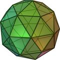
Archimedean and Catalan solids
Conway's original set of operators can create all of the Archimedean solids and Catalan solids, using the Platonic solids as seeds. (Note that the r operator is not necessary to create both chiral forms.)
- Archimedean
Cuboctahedron
aC = aO = eT
Truncated octahedron
tO = bT
Rhombicuboctahedron
eC = eO
truncated cuboctahedron
bC = bO
snub cube
sC = sO
icosidodecahedron
aD = aI
rhombicosidodecahedron
eD = eI
truncated icosidodecahedron
bD = bI
snub dodecahedron
sD = sI


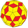
- Catalan
Rhombic dodecahedron
jC = jO = oT
Tetrakis hexahedron
kC = mT
Deltoidal icositetrahedron
oC = oO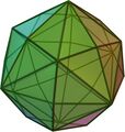
Disdyakis dodecahedron
mC = mO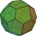
Pentagonal icositetrahedron
gC = gO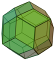
Rhombic triacontahedron
jD = jI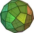
Deltoidal hexecontahedron
oD = oI
Disdyakis triacontahedron
mD = mI
Pentagonal hexecontahedron
gD = gI


Composite operators
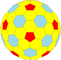
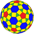
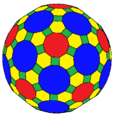
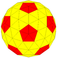
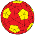
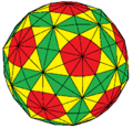
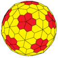
The truncated icosahedron, tI, can be used as a seed to create some more visually-pleasing polyhedra, although these are neither vertex nor face-transitive.
tI
atI
ttI
ztI = ttD
etI
btI
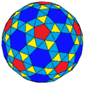
stI


- Duals
dtI = nI = kD
jtI
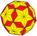
ntI = kkD
ktI
otI
mtI
gtI


On the plane
Each of the convex uniform tilings and their duals can be created by applying Conway operators to the regular tilings Q, H, and Δ.
Square tiling
Q = dQ = aQ = eQ
= jQ = oQ
Truncated square tiling
tQ = bQ
Tetrakis square tiling
kQ = mQ


Hexagonal tiling
H = dΔ = tΔ
Trihexagonal tiling
aH = aΔ
Rhombitrihexagonal tiling
eH = eΔ
Snub trihexagonal tiling
sH = sΔ


Triangle tiling
Δ = dH = kH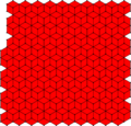
Rhombille tiling
jΔ = jH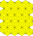
Triakis triangular tiling
kΔ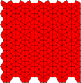
Deltoidal trihexagonal tiling
oΔ = oH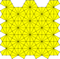
Kisrhombille tiling
mΔ = mH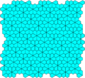
Floret pentagonal tiling
gΔ = gH


On a torus
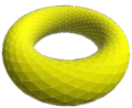
Conway operators can also be applied to toroidal polyhedra and polyhedra with multiple holes.
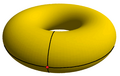
A 1x1 regular square torus, {4,4}1,0
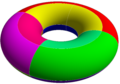
A regular 4x4 square torus, {4,4}4,0
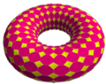
tQ24×12 projected to torus
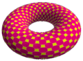
taQ24×12 projected to torus
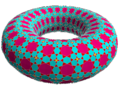
actQ24×8 projected to torus
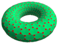
tH24×12 projected to torus
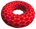
taH24×8 projected to torus
kH24×12 projected to torus


See also
| Wikimedia Commons has media related to Conway polyhedra. |
References
- ↑ "Chapter 21: Naming Archimedean and Catalan polyhedra and tilings". The Symmetries of Things. AK Peters. 2008. p. 288. ISBN 978-1-56881-220-5.
- ↑ Weisstein, Eric W.. "Conway Polyhedron Notation". http://mathworld.wolfram.com/ConwayPolyhedronNotation.html.
- ↑ 3.0 3.1 George W. Hart (1998). "Conway Notation for Polyhedra". http://www.georgehart.com/virtual-polyhedra/conway_notation.html.
- ↑ 4.0 4.1 4.2 4.3 4.4 Adrian Rossiter. "conway - Conway Notation transformations". http://www.antiprism.com/programs/conway.html.
- ↑ Anselm Levskaya. "polyHédronisme". https://levskaya.github.io/polyhedronisme/.
- ↑ 6.0 6.1 Hart, George (1998). "Conway Notation for Polyhedra". http://www.georgehart.com/virtual-polyhedra/conway_notation.html. (See fourth row in table, "a = ambo".)
- ↑ 7.0 7.1 7.2 Brinkmann, G.; Goetschalckx, P.; Schein, S. (2017). "Goldberg, Fuller, Caspar, Klug and Coxeter and a general approach to local symmetry-preserving operations". Proceedings of the Royal Society A: Mathematical, Physical and Engineering Sciences 473 (2206): 20170267. doi:10.1098/rspa.2017.0267. Bibcode: 2017RSPSA.47370267B.
- ↑ 8.0 8.1 Goetschalckx, Pieter; Coolsaet, Kris; Van Cleemput, Nico (2020-04-12). "Generation of Local Symmetry-Preserving Operations". arXiv:1908.11622 [math.CO].
- ↑ Goetschalckx, Pieter; Coolsaet, Kris; Van Cleemput, Nico (2020-04-11). "Local Orientation-Preserving Symmetry Preserving Operations on Polyhedra". arXiv:2004.05501 [math.CO].
- ↑ Weisstein, Eric W.. "Rectification". http://mathworld.wolfram.com/Rectification.html.
- ↑ Weisstein, Eric W.. "Cumulation". http://mathworld.wolfram.com/Cumulation.html.
- ↑ Weisstein, Eric W.. "Truncation". http://mathworld.wolfram.com/Truncation.html.
- ↑ "Antiprism - Chirality issue in conway". https://groups.google.com/forum/#!topic/antiprism/6NcYnKP4mTc.
- ↑ Livio Zefiro (2008). "Generation of an icosahedron by the intersection of five tetrahedra: geometrical and crystallographic features of the intermediate polyhedra". Vismath. http://www.mi.sanu.ac.rs/vismath/zefiro2008/__generation_of_icosahedron_by_5tetrahedra.htm.
- ↑ George W. Hart (August 2000). "Sculpture based on Propellorized Polyhedra". Proceedings of MOSAIC 2000. Seattle, WA. pp. 61–70. http://www.georgehart.com/propello/propello.html.
- ↑ Deza, M.; Dutour, M (2004). "Goldberg–Coxeter constructions for 3-and 4-valent plane graphs". The Electronic Journal of Combinatorics 11: #R20. doi:10.37236/1773. http://www.combinatorics.org/ojs/index.php/eljc/article/view/v11i1r20.
- ↑ Deza, M.-M.; Sikirić, M. D.; Shtogrin, M. I. (2015). "Goldberg–Coxeter Construction and Parameterization". Geometric Structure of Chemistry-Relevant Graphs: Zigzags and Central Circuits. Springer. pp. 131–148. ISBN 9788132224495. https://books.google.com/books?id=HLi4CQAAQBAJ&q=goldberg-coxeter&pg=PA130.
External links
- polyHédronisme: generates polyhedra in HTML5 canvas, taking Conway notation as input
 |  |

