Chambolle-Pock algorithm
In mathematics, the Chambolle-Pock algorithm is an algorithm used to solve convex optimization problems. It was introduced by Antonin Chambolle and Thomas Pock[1] in 2011 and has since become a widely used method in various fields, including image processing,[2][3][4] computer vision,[5] and signal processing.[6]
The Chambolle-Pock algorithm is specifically designed to efficiently solve convex optimization problems that involve the minimization of a non-smooth cost function composed of a data fidelity term and a regularization term.[1] This is a typical configuration that commonly arises in ill-posed imaging inverse problems such as image reconstruction,[2] denoising[3] and inpainting.[4]
The algorithm is based on a primal-dual formulation, which allows for simultaneous updates of primal and dual variables. By employing the proximal operator, the Chambolle-Pock algorithm efficiently handles non-smooth and non-convex regularization terms, such as the total variation, specific in imaging framework.[1]
Problem statement
Let be two real vector spaces equipped with an inner product and a norm . From up to now, a function is called simple if its proximal operator has a closed-form representation or can be accurately computed, for ,[1] where is referred to
Consider the following constrained primal problem:[1]
where is a bounded linear operator, are convex, lower semicontinuous and simple.[1]
The minimization problem has its dual corresponding problem as[1]
where and are the dual map of and , respectively.[1]
Assume that the primal and the dual problems have at least a solution , that means they satisfies[7]
where and are the subgradient of the convex functions and , respectively.[7]
The Chambolle-Pock algorithm solves the so-called saddle-point problem[1]
which is a primal-dual formulation of the nonlinear primal and dual problems stated before.[1]
Algorithm
The Chambolle-Pock algorithm primarily involves iteratively alternating between ascending in the dual variable
and descending in the primal variable
using a gradient-like approach, with step sizes
and
respectively, in order to simultaneously solve the primal and the dual problem.[2] Furthermore, an over-relaxation technique is employed for the primal variable with the parameter
.[1]
Algorithm Chambolle-Pock algorithm
Input: and set , stopping criterion.
do while stopping criterion not satisfied
end do
- "←" denotes assignment. For instance, "largest ← item" means that the value of largest changes to the value of item.
- "return" terminates the algorithm and outputs the following value.
Chambolle and Pock proved[1] that the algorithm converges if and , sequentially and with as rate of convergence for the primal-dual gap. This has been extended by S. Banert et al.[8] to hold whenever and .
The semi-implicit Arrow-Hurwicz method[9] coincides with the particular choice of in the Chambolle-Pock algorithm.[1]
Acceleration
There are special cases in which the rate of convergence has a theoretical speed up.[1] In fact, if , respectively , is uniformly convex then , respectively , has a Lipschitz continuous gradient. Then, the rate of convergence can be improved to , providing a slightly changes in the Chambolle-Pock algorithm. It leads to an accelerated version of the method and it consists in choosing iteratively , and also , instead of fixing these values.[1]
In case of uniformly convex, with the uniform-convexity constant, the modified algorithm becomes[1]
Algorithm Accelerated Chambolle-Pock algorithm
Input: such that and set , stopping criterion.
do while stopping criterion not satisfied
end do
- "←" denotes assignment. For instance, "largest ← item" means that the value of largest changes to the value of item.
- "return" terminates the algorithm and outputs the following value.
Moreover, the convergence of the algorithm slows down when , the norm of the operator , cannot be estimated easily or might be very large. Choosing proper preconditioners and , modifying the proximal operator with the introduction of the induced norm through the operators and , the convergence of the proposed preconditioned algorithm will be ensured.[10]
Application
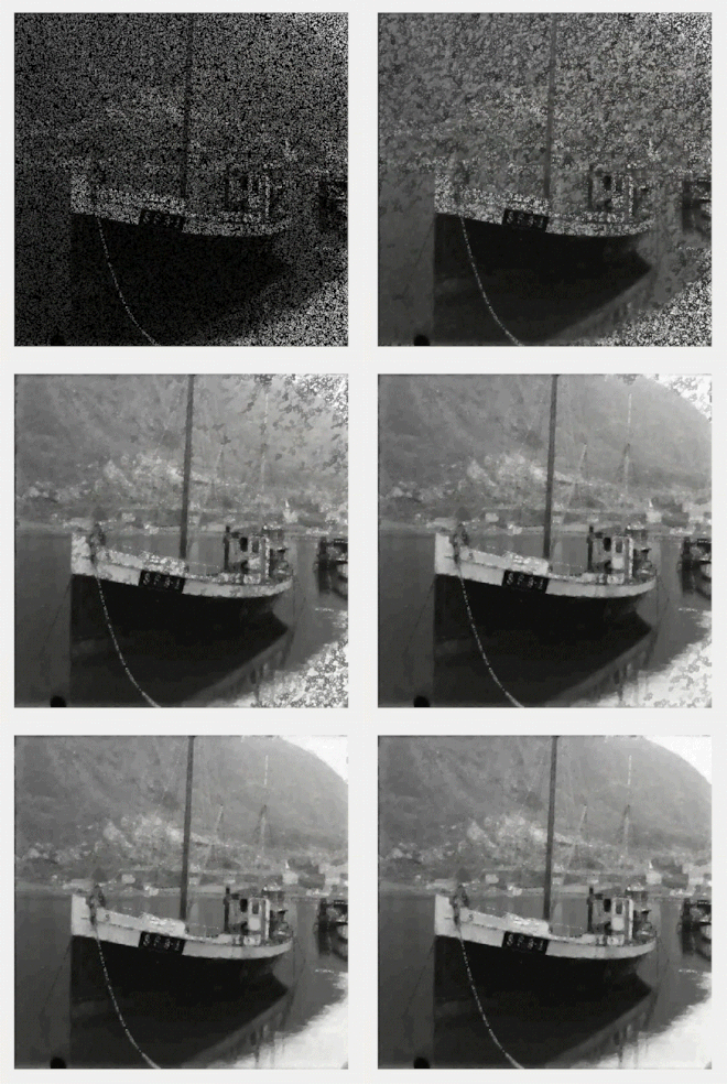
A typical application of this algorithm is in the image denoising framework, based on total variation.[3] It operates on the concept that signals containing excessive and potentially erroneous details exhibit a high total variation, which represents the integral of the absolute value gradient of the image.[3] By adhering to this principle, the process aims to decrease the total variation of the signal while maintaining its similarity to the original signal, effectively eliminating unwanted details while preserving crucial features like edges. In the classical bi-dimensional discrete setting,[11] consider , where an element represents an image with the pixels values collocated in a Cartesian grid .[1]
Define the inner product on as[1]
that induces an norm on , denoted as .[1]
Hence, the gradient of is computed with the standard finite differences,
which is an element of the space , where[1]
On is defined an based norm as[1]
Then, the primal problem of the ROF model, proposed by Rudin, Osher, and Fatemi,[12] is given by[1]
where is the unknown solution and the given noisy data, instead describes the trade-off between regularization and data fitting.[1]
The primal-dual formulation of the ROF problem is formulated as follow[1]
where the indicator function is defined as[1]
on the convex set which can be seen as unitary balls with respect to the defined norm on .[1]
Observe that the functions involved in the stated primal-dual formulation are simple, since their proximal operator can be easily computed[1]The image total-variation denoising problem can be also treated with other algorithms[13] such as the alternating direction method of multipliers (ADMM),[14] projected (sub)-gradient[15] or fast iterative shrinkage thresholding.[16]
Implementation
- The Manopt.jl[17] package implements the algorithm in Julia
- Gabriel Peyré implements the algorithm in MATLAB,[note 1] Julia, R and Python[18]
- In the Operator Discretization Library (ODL),[19] a Python library for inverse problems,
chambolle_pock_solverimplements the method.
See also
- Alternating direction method of multipliers
- Convex optimization
- Proximal operator
- Total variation denoising
Notes
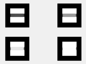
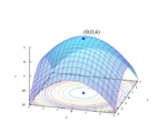
- ↑ These codes were used to obtain the images in the article.
References
- ↑ 1.00 1.01 1.02 1.03 1.04 1.05 1.06 1.07 1.08 1.09 1.10 1.11 1.12 1.13 1.14 1.15 1.16 1.17 1.18 1.19 1.20 1.21 1.22 1.23 1.24 1.25 1.26 Chambolle, Antonin; Pock, Thomas (2011-05-01). "A First-Order Primal-Dual Algorithm for Convex Problems with Applications to Imaging" (in en). Journal of Mathematical Imaging and Vision 40 (1): 120–145. doi:10.1007/s10851-010-0251-1. ISSN 1573-7683. https://doi.org/10.1007/s10851-010-0251-1.
- ↑ 2.0 2.1 2.2 Sidky, Emil Y; Jørgensen, Jakob H; Pan, Xiaochuan (2012-05-21). "Convex optimization problem prototyping for image reconstruction in computed tomography with the Chambolle–Pock algorithm". Physics in Medicine and Biology 57 (10): 3065–3091. doi:10.1088/0031-9155/57/10/3065. ISSN 0031-9155. PMID 22538474. Bibcode: 2012PMB....57.3065S.
- ↑ 3.0 3.1 3.2 3.3 Fang, Faming; Li, Fang; Zeng, Tieyong (2014-03-13). "Single Image Dehazing and Denoising: A Fast Variational Approach" (in en). SIAM Journal on Imaging Sciences 7 (2): 969–996. doi:10.1137/130919696. ISSN 1936-4954. http://epubs.siam.org/doi/10.1137/130919696.
- ↑ 4.0 4.1 Allag, A.; Benammar, A.; Drai, R.; Boutkedjirt, T. (2019-07-01). "Tomographic Image Reconstruction in the Case of Limited Number of X-Ray Projections Using Sinogram Inpainting" (in en). Russian Journal of Nondestructive Testing 55 (7): 542–548. doi:10.1134/S1061830919070027. ISSN 1608-3385. https://doi.org/10.1134/S1061830919070027.
- ↑ Pock, Thomas; Cremers, Daniel; Bischof, Horst; Chambolle, Antonin (2009). "An algorithm for minimizing the Mumford-Shah functional". 2009 IEEE 12th International Conference on Computer Vision. pp. 1133–1140. doi:10.1109/ICCV.2009.5459348. ISBN 978-1-4244-4420-5. https://ieeexplore.ieee.org/document/5459348.
- ↑ "A Generic Proximal Algorithm for Convex Optimization—Application to Total Variation Minimization". IEEE Signal Processing Letters 21 (8): 985–989. 2014. doi:10.1109/LSP.2014.2322123. ISSN 1070-9908. Bibcode: 2014ISPL...21..985.. https://ieeexplore.ieee.org/document/6810809.
- ↑ 7.0 7.1 Ekeland, Ivar; Témam, Roger (1999) (in en). Convex Analysis and Variational Problems. Society for Industrial and Applied Mathematics. p. 61. doi:10.1137/1.9781611971088. ISBN 978-0-89871-450-0. http://epubs.siam.org/doi/book/10.1137/1.9781611971088.
- ↑ Banert, Sebastian; Upadhyaya, Manu; Giselsson, Pontus (2023). "The Chambolle-Pock method converges weakly with and ". arXiv:2309.03998 [math.OC].
- ↑ Uzawa, H. (1958). "Iterative methods for concave programming". in Arrow, K. J.; Hurwicz, L.; Uzawa, H.. Studies in linear and nonlinear programming. Stanford University Press. https://archive.org/details/studiesinlinearn0000arro.
- ↑ Pock, Thomas; Chambolle, Antonin (2011-11-06). "Diagonal preconditioning for first order primal-dual algorithms in convex optimization". 2011 International Conference on Computer Vision. pp. 1762–1769. doi:10.1109/ICCV.2011.6126441. ISBN 978-1-4577-1102-2. https://ieeexplore.ieee.org/document/6126441.
- ↑ Chambolle, Antonin (2004-01-01). "An Algorithm for Total Variation Minimization and Applications" (in en). Journal of Mathematical Imaging and Vision 20 (1): 89–97. doi:10.1023/B:JMIV.0000011325.36760.1e. ISSN 1573-7683. https://doi.org/10.1023/B:JMIV.0000011325.36760.1e.
- ↑ Getreuer, Pascal (2012). "Rudin–Osher–Fatemi Total Variation Denoising using Split Bregman". https://www.ipol.im/pub/art/2012/g-tvd/article_lr.pdf.
- ↑ Esser, Ernie; Zhang, Xiaoqun; Chan, Tony F. (2010). "A General Framework for a Class of First Order Primal-Dual Algorithms for Convex Optimization in Imaging Science" (in en). SIAM Journal on Imaging Sciences 3 (4): 1015–1046. doi:10.1137/09076934X. ISSN 1936-4954. http://epubs.siam.org/doi/10.1137/09076934X.
- ↑ Lions, P. L.; Mercier, B. (1979). "Splitting Algorithms for the Sum of Two Nonlinear Operators". SIAM Journal on Numerical Analysis 16 (6): 964–979. doi:10.1137/0716071. ISSN 0036-1429. Bibcode: 1979SJNA...16..964L. https://www.jstor.org/stable/2156649.
- ↑ Beck, Amir; Teboulle, Marc (2009). "A Fast Iterative Shrinkage-Thresholding Algorithm for Linear Inverse Problems" (in en). SIAM Journal on Imaging Sciences 2 (1): 183–202. doi:10.1137/080716542. ISSN 1936-4954. http://epubs.siam.org/doi/10.1137/080716542.
- ↑ Nestorov, Yu.E.. "A method of solving a convex programming problem with convergence rate ". Dokl. Akad. Nauk SSSR 269 (3): 543–547. https://www.mathnet.ru/eng/dan46009.
- ↑ "Chambolle-Pock · Manopt.jl" (in en). https://docs.juliahub.com/Manopt/h1Pdc/0.3.8/solvers/ChambollePock.html.
- ↑ "Numerical Tours - A Numerical Tour of Data Science". http://www.numerical-tours.com/.
- ↑ "Chambolle-Pock solver — odl 0.6.1.dev0 documentation". https://odl.readthedocs.io/guide/chambolle_pock_guide.html#chambolle-pock-guide.
Further reading
- Boyd, Stephen; Vandenberghe, Lieven (2004). Convex Optimization. Cambridge University Press. https://web.stanford.edu/~boyd/cvxbook/bv_cvxbook.pdf.
- Wright, Stephen (1997). Primal-Dual Interior-Point Methods. Philadelphia, PA: SIAM. ISBN 978-0-89871-382-4.
- Nocedal, Jorge; Stephen Wright (1999). Numerical Optimization. New York, NY: Springer. ISBN 978-0-387-98793-4.
External links
- EE364b, a Stanford course homepage.


