Path analysis (statistics)

In statistics, path analysis is used to describe the directed dependencies among a set of variables. This includes models equivalent to any form of multiple regression analysis, factor analysis, canonical correlation analysis, discriminant analysis, as well as more general families of models in the multivariate analysis of variance and covariance analyses (MANOVA, ANOVA, ANCOVA). In addition to being thought of as a form of multiple regression focusing on causality, path analysis can be viewed as a special case of structural equation modeling (SEM) – one in which only single indicators are employed for each of the variables in the causal model. That is, path analysis is SEM with a structural model, but no measurement model. Other terms used to refer to path analysis include causal modeling and analysis of covariance structures.

Path analysis is considered by Judea Pearl to be a direct ancestor to the techniques of Causal inference.

History

Path analysis was developed around 1918 by geneticist Sewall Wright, who wrote about it more extensively in the 1920s. It has since been applied to a vast array of complex modeling areas, including biology, psychology, sociology, and econometrics.

Path modeling

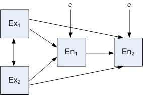
Typically, path models consist of independent and dependent variables depicted graphically by boxes or rectangles. Variables that are independent variables, and not dependent variables, are called 'exogenous'. Graphically, these exogenous variable boxes lie at outside edges of the model and have only single-headed arrows exiting from them. No single-headed arrows point at exogenous variables. Variables that are solely dependent variables, or are both independent and dependent variables, are termed 'endogenous'. Graphically, endogenous variables have at least one single-headed arrow pointing at them.

In the model below, the two exogenous variables (Ex₁ and Ex₂) are modeled as being correlated as depicted by the double-headed arrow. Both of these variables have direct and indirect (through En₁) effects on En₂ (the two dependent or 'endogenous' variables/factors). In most real-world models, the endogenous variables may also be affected by variables and factors stemming from outside the model (external effects including measurement error). These effects are depicted by the "e" or error terms in the model.

Using the same variables, alternative models are conceivable. For example, it may be hypothesized that Ex₁ has only an indirect effect on En₂, deleting the arrow from Ex₁ to En₂; and the likelihood or 'fit' of these two models can be compared statistically.

Path tracing rules

In order to validly calculate the relationship between any two boxes in the diagram, Wright (1934) proposed a simple set of path tracing rules, for calculating the correlation between two variables. The correlation is equal to the sum of the contribution of all the pathways through which the two variables are connected. The strength of each of these contributing pathways is calculated as the product of the path-coefficients along that pathway.

The rules for path tracing are:

1. You can trace backward up an arrow and then forward along the next, or forwards from one variable to the other, but never forward and then back. Another way to think of this rule is that you can never pass out of one arrow head and into another arrowhead: heads-tails, or tails-heads, not heads-heads.
2. You can pass through each variable only once in a given chain of paths.
3. No more than one bi-directional arrow can be included in each path-chain.

Again, the expected correlation due to each chain traced between two variables is the product of the standardized path coefficients, and the total expected correlation between two variables is the sum of these contributing path-chains.

NB: Wright's rules assume a model without feedback loops: the directed graph of the model must contain no cycles, i.e. it is a directed acyclic graph, which has been extensively studied in the causal analysis framework of Judea Pearl.

Path tracing in unstandardized models

If the modeled variables have not been standardized, an additional rule allows the expected covariances to be calculated as long as no paths exist connecting dependent variables to other dependent variables.

The simplest case obtains where all residual variances are modeled explicitly. In this case, in addition to the three rules above, calculate expected covariances by:

1. Compute the product of coefficients in each route between the variables of interest, tracing backwards, changing direction at a two-headed arrow, then tracing forwards.
2. Sum over all distinct routes, where pathways are considered distinct if they contain different coefficients, or encounter those coefficients in a different order.

Where residual variances are not explicitly included, or as a more general solution, at any change of direction encountered in a route (except for at two-way arrows), include the variance of the variable at the point of change. That is, in tracing a path from a dependent variable to an independent variable, include the variance of the independent-variable except where so doing would violate rule 1 above (passing through adjacent arrowheads: i.e., when the independent variable also connects to a double-headed arrow connecting it to another independent variable). In deriving variances (which is necessary in the case where they are not modeled explicitly), the path from a dependent variable into an independent variable and back is counted once only.

See also

• Bayesian network
• Causality
• Causal loop diagram
• Hidden Markov model
• Latent variable model
• Path coefficient
• Structural equation model (SEM)

External links

• Ωnyx, a free software environment for Structural Equation Modeling
• OpenMx - Advanced Structural Equation Modeling
• LISREL: model, methods and software for Structural Equation Modeling

References

- ↑ Pearl, Judea (May 2018). The Book of Why. New York: Basic Books. p. 6. ISBN 978-0-465-09760-9.
- ↑ Wright, S. (1921). "Correlation and causation". J. Agricultural Research 20: 557–585.
- ↑ Dodge, Y. (2003) The Oxford Dictionary of Statistical Terms. OUP. ISBN 0-19-920613-9
- ↑ Wright, S. (1934). "The method of path coefficients". Annals of Mathematical Statistics 5 (3): 161–215. doi:10.1214/aoms/1177732676.