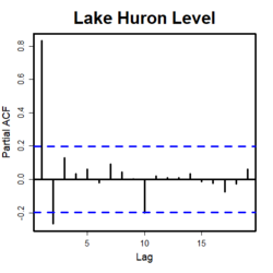
Partial autocorrelation function

In time series analysis, the partial autocorrelation function (PACF) gives the partial correlation of a stationary time series with its own lagged values, regressed the values of the time series at all shorter lags. It contrasts with the autocorrelation function, which does not control for other lags.
This function plays an important role in data analysis aimed at identifying the extent of the lag in an autoregressive (AR) model. The use of this function was introduced as part of the Box–Jenkins approach to time series modelling, whereby plotting the partial autocorrelative functions one could determine the appropriate lags p in an AR (p) model or in an extended ARIMA (p,d,q) model.
Definition
Given a time series , the partial autocorrelation of lag , denoted , is the autocorrelation between and with the linear dependence of on through removed. Equivalently, it is the autocorrelation between and that is not accounted for by lags through , inclusive.[1]where and are linear combinations of that minimize the mean squared error of and respectively. For stationary processes, the coefficients in and are the same, but reversed:[2]
Calculation
The theoretical partial autocorrelation function of a stationary time series can be calculated by using the Durbin–Levinson Algorithm:where for and is the autocorrelation function.[3][4][5]
The formula above can be used with sample autocorrelations to find the sample partial autocorrelation function of any given time series.[6][7]
Examples
The following table summarizes the partial autocorrelation function of different models:[5][8]
| Model | PACF |
|---|---|
| White noise | The partial autocorrelation is 0 for all lags. |
| Autoregressive model | The partial autocorrelation for an AR(p) model is nonzero for lags less than or equal to p and 0 for lags greater than p. |
| Moving-average model | If , the partial autocorrelation oscillates to 0. |
| If , the partial autocorrelation geometrically decays to 0. | |
| Autoregressive–moving-average model | An ARMA(p, q) model's partial autocorrelation geometrically decays to 0 but only after lags greater than p. |
The behavior of the partial autocorrelation function mirrors that of the autocorrelation function for autoregressive and moving-average models. For example, the partial autocorrelation function of an AR(p) series cuts off after lag p similar to the autocorrelation function of an MA(q) series with lag q. In addition, the autocorrelation function of an AR(p) process tails off just like the partial autocorrelation function of an MA(q) process.[2]
Autoregressive model identification

Partial autocorrelation is a commonly used tool for identifying the order of an autoregressive model.[6] As previously mentioned, the partial autocorrelation of an AR(p) process is zero at lags greater than p.[5][8] If an AR model is determined to be appropriate, then the sample partial autocorrelation plot is examined to help identify the order.
The partial autocorrelation of lags greater than p for an AR(p) time series are approximately independent and normal with a mean of 0.[9] Therefore, a confidence interval can be constructed by dividing a selected z-score by . Lags with partial autocorrelations outside of the confidence interval indicate that the AR model's order is likely greater than or equal to the lag. Plotting the partial autocorrelation function and drawing the lines of the confidence interval is a common way to analyze the order of an AR model. To evaluate the order, one examines the plot to find the lag after which the partial autocorrelations are all within the confidence interval. This lag is determined to likely be the AR model's order.[1]
References
- ↑ 1.0 1.1 "6.4.4.6.3. Partial Autocorrelation Plot". https://www.itl.nist.gov/div898/handbook/pmc/section4/pmc4463.htm.
- ↑ 2.0 2.1 Shumway, Robert H.; Stoffer, David S. (2017) (in en). Time Series Analysis and Its Applications: With R Examples. Springer Texts in Statistics. Cham: Springer International Publishing. pp. 97–99. doi:10.1007/978-3-319-52452-8. ISBN 978-3-319-52451-1. http://link.springer.com/10.1007/978-3-319-52452-8.
- ↑ Durbin, J. (1960). "The Fitting of Time-Series Models". Revue de l'Institut International de Statistique / Review of the International Statistical Institute 28 (3): 233–244. doi:10.2307/1401322. ISSN 0373-1138. https://www.jstor.org/stable/1401322.
- ↑ Shumway, Robert H.; Stoffer, David S. (2017) (in en). Time Series Analysis and Its Applications: With R Examples. Springer Texts in Statistics. Cham: Springer International Publishing. pp. 103–104. doi:10.1007/978-3-319-52452-8. ISBN 978-3-319-52451-1. http://link.springer.com/10.1007/978-3-319-52452-8.
- ↑ 5.0 5.1 5.2 Enders, Walter (2004) (in en). Applied econometric time series (2nd ed.). Hoboken, NJ: J. Wiley. pp. 65–67. ISBN 0-471-23065-0. OCLC 52387978.
- ↑ 6.0 6.1 Box, George E. P.; Reinsel, Gregory C.; Jenkins, Gwilym M. (2008) (in en). Time Series Analysis: Forecasting and Control (4th ed.). Hoboken, New Jersey: John Wiley. ISBN 9780470272848.
- ↑ Brockwell, Peter J.; Davis, Richard A. (1991) (in en). Time Series: Theory and Methods (2nd ed.). New York, NY: Springer. pp. 102, 243–245. ISBN 9781441903198.
- ↑ 8.0 8.1 Das, Panchanan (2019) (in en). Econometrics in Theory and Practice : Analysis of Cross Section, Time Series and Panel Data with Stata 15. 1. Singapore: Springer. pp. 294–299. ISBN 978-981-329-019-8. OCLC 1119630068.
- ↑ Quenouille, M. H. (1949). "Approximate Tests of Correlation in Time-Series" (in en). Journal of the Royal Statistical Society, Series B (Methodological) 11 (1): 68–84. doi:10.1111/j.2517-6161.1949.tb00023.x. https://onlinelibrary.wiley.com/doi/10.1111/j.2517-6161.1949.tb00023.x.
 |
