Graphical model

Short description: Probabilistic model

A graphical model or probabilistic graphical model (PGM) or structured probabilistic model is a probabilistic model for which a graph expresses the conditional dependence structure between random variables. They are commonly used in probability theory, statistics—particularly Bayesian statistics—and machine learning.

Types of graphical models

Generally, probabilistic graphical models use a graph-based representation as the foundation for encoding a distribution over a multi-dimensional space and a graph that is a compact or factorized representation of a set of independences that hold in the specific distribution. Two branches of graphical representations of distributions are commonly used, namely, Bayesian networks and Markov random fields. Both families encompass the properties of factorization and independences, but they differ in the set of independences they can encode and the factorization of the distribution that they induce.

Undirected Graphical Model

An undirected graph with four vertices.

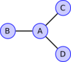
The undirected graph shown may have one of several interpretations; the common feature is that the presence of an edge implies some sort of dependence between the corresponding random variables. From this graph we might deduce that [math]\displaystyle{ B,C,D }[/math] are all mutually independent, once [math]\displaystyle{ A }[/math] is known, or (equivalently in this case) that

[math]\displaystyle{ P[A,B,C,D] = f_{AB}[A,B] \cdot f_{AC}[A,C] \cdot f_{AD}[A,D] }[/math]

for some non-negative functions [math]\displaystyle{ f_{AB}, f_{AC}, f_{AD} }[/math].

Bayesian network

Example of a directed acyclic graph on four vertices.

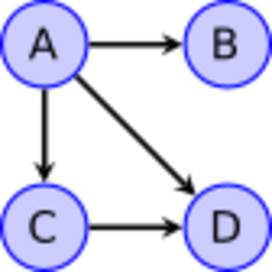
If the network structure of the model is a directed acyclic graph, the model represents a factorization of the joint probability of all random variables. More precisely, if the events are [math]\displaystyle{ X_1,\ldots,X_n }[/math] then the joint probability satisfies

[math]\displaystyle{ P[X_1,\ldots,X_n]=\prod_{i=1}^nP[X_i|\text{pa}(X_i)] }[/math]

where [math]\displaystyle{ \text{pa}(X_i) }[/math] is the set of parents of node [math]\displaystyle{ X_i }[/math] (nodes with edges directed towards [math]\displaystyle{ X_i }[/math]). In other words, the joint distribution factors into a product of conditional distributions. For example, in the directed acyclic graph shown in the Figure this factorization would be

[math]\displaystyle{ P[A,B,C,D] = P[A]\cdot P[B | A]\cdot P[C | A] \cdot P[D|A,C] }[/math].

Any two nodes are conditionally independent given the values of their parents. In general, any two sets of nodes are conditionally independent given a third set if a criterion called d-separation holds in the graph. Local independences and global independences are equivalent in Bayesian networks.

This type of graphical model is known as a directed graphical model, Bayesian network, or belief network. Classic machine learning models like hidden Markov models, neural networks and newer models such as variable-order Markov models can be considered special cases of Bayesian networks.

One of the simplest Bayesian Networks is the Naive Bayes classifier.

Cyclic Directed Graphical Models

An example of a directed, cyclic graphical model. Each arrow indicates a dependency. In this example: D depends on A, B, and C; and C depends on B and D; whereas A and B are each independent.

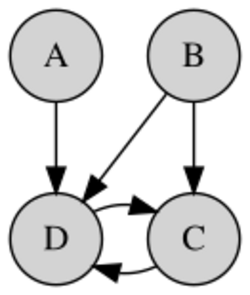
The next figure depicts a graphical model with a cycle. This may be interpreted in terms of each variable 'depending' on the values of its parents in some manner. The particular graph shown suggests a joint probability density that factors as

[math]\displaystyle{ P[A,B,C,D] = P[A]\cdot P[B]\cdot P[C,D|A,B] }[/math],

but other interpretations are possible.

Other types

• Dependency network where cycles are allowed
• Tree-augmented classifier or TAN model

TAN model for "corral dataset".

• Targeted Bayesian network learning (TBNL)
  

  TBNL model for "corral dataset"
• A factor graph is an undirected bipartite graph connecting variables and factors. Each factor represents a function over the variables it is connected to. This is a helpful representation for understanding and implementing belief propagation.
• A clique tree or junction tree is a tree of cliques, used in the junction tree algorithm.
• A chain graph is a graph which may have both directed and undirected edges, but without any directed cycles (i.e. if we start at any vertex and move along the graph respecting the directions of any arrows, we cannot return to the vertex we started from if we have passed an arrow). Both directed acyclic graphs and undirected graphs are special cases of chain graphs, which can therefore provide a way of unifying and generalizing Bayesian and Markov networks.
• An ancestral graph is a further extension, having directed, bidirected and undirected edges.
• Random field techniques
  • A Markov random field, also known as a Markov network, is a model over an undirected graph. A graphical model with many repeated subunits can be represented with plate notation.
  • A conditional random field is a discriminative model specified over an undirected graph.
• A restricted Boltzmann machine is a bipartite generative model specified over an undirected graph.

Applications

The framework of the models, which provides algorithms for discovering and analyzing structure in complex distributions to describe them succinctly and extract the unstructured information, allows them to be constructed and utilized effectively. Applications of graphical models include causal inference, information extraction, speech recognition, computer vision, decoding of low-density parity-check codes, modeling of gene regulatory networks, gene finding and diagnosis of diseases, and graphical models for protein structure.

See also

• Belief propagation
• Structural equation model

Further reading

Books and book chapters

• Barber, David (2012). Bayesian Reasoning and Machine Learning. Cambridge University Press. ISBN 978-0-521-51814-7. 

• Bishop, Christopher M. (2006). "Chapter 8. Graphical Models". Pattern Recognition and Machine Learning. Springer. pp. 359–422. ISBN 978-0-387-31073-2. https://www.microsoft.com/en-us/research/wp-content/uploads/2016/05/Bishop-PRML-sample.pdf. 
• {{cite book

|author=Cowell, Robert G.

• Jensen, Finn (1996). An introduction to Bayesian networks. Berlin: Springer. ISBN 978-0-387-91502-9. 
• Probabilistic Reasoning in Intelligent Systems (2nd revised ed.). San Mateo, CA: Morgan Kaufmann. 1988. ISBN 978-1-55860-479-7. https://archive.org/details/probabilisticrea00pear.  A computational reasoning approach, where the relationships between graphs and probabilities were formally introduced.

Journal articles

• "Getting Started in Probabilistic Graphical Models". PLOS Computational Biology 3 (12): e252. 2007. doi:10.1371/journal.pcbi.0030252. PMID 18069887. Bibcode: 2007PLSCB...3..252A. 
• Jordan, M. I. (2004). "Graphical Models". Statistical Science 19: 140–155. doi:10.1214/088342304000000026. 
• Ghahramani, Zoubin (May 2015). "Probabilistic machine learning and artificial intelligence" (in en). Nature 521 (7553): 452–459. doi:10.1038/nature14541. PMID 26017444. Bibcode: 2015Natur.521..452G. https://www.repository.cam.ac.uk/handle/1810/248538. 

Other

• Heckerman's Bayes Net Learning Tutorial
• A Brief Introduction to Graphical Models and Bayesian Networks
• Sargur Srihari's lecture slides on probabilistic graphical models

External links

• Graphical models and Conditional Random Fields
• Probabilistic Graphical Models taught by Eric Xing at CMU